Models Comparison To Assess Emerging Of Low Income Housing In Colombo Suburbs

Abstract

The Colombo Metropolitan Region is the economic powerhouse of the whole country, with vigorous commercial and industrial activities. Over the past few decades, its low-lying areas have been undergoing drastic changes. All factors relating to this have been considered by studying three sectorial models and an overall model. In the sectorial models, several variables / factors affecting conversion of low-lying housing plots have been identified, but the important need is to pinpoint the most influential variables. This is determined using the overall model and the three sectorial models. The overall model considers 19 variables in all but excludes family savings (because of its multicollinearity with family income). Of the 19 variables in the overall model, 8 variables proved significant. It was found that three variables from the Geo-spatial group (RWR, GWS & LLP), three variables from the Behaviour group (PPP, TSA & PPG) and two variables from the socio-economic group (HI & SKJ) proved significant in the overall model, showing high levels of accuracy in each model. Hence, in the context of low-lying land conversion the most influential variables are the geo-spatial and behaviour variables as proved both statistically and empirically. As such, the overall model has conclusively identified the most influential variables that exerted the greatest impact on low-lying land conversion, by causing the emergence of households. All data from models along with their probability values have been mapped using GIS to understand the levels of conversion that took place in the low-lying areas of Colombo Metropolitan Region.

Keywords: Geo-StatisticGIShousingsettlementsuburbanurban planning

Introduction

It is acknowledged by town and city planners that the utilization and conversion of land are primarily influenced by the factors of time, space and human interactions. For example, it can be seen that civil works such as concrete highways, asphalt roads, factories, industrial sites and housing developments are densely scattered across environmentally sensitive low-lying lands including marshes and paddy fields that have been filled in. Colombo and its suburbs have now become heavily built-up areas with a preponderance of individual housing units occupying practically all the low-lying areas (Samaratunga & O'Hare, 2013). As mentioned earlier, this has been an on-going process that has eventually resulted in the takeover of every available plot in the low-lying areas and its gradual transformation into a stable homestead. The conversion of land occurs very slowly at first but the process gains momentum later on until every vacant plot of land is acquired and occupied. This uncontrolled growth ultimately leads to urban chaos on several fronts (Dayaratne, 2010).

Problem Statement

Changes to low-lying areas that occurred over the period under review can be made visible as hot spots across the entire area covered by the CMR using spatial techniques. One of the tasks of the study was to find out, “Where are the low-lying areas that are still being threatened by the emergence of new households?” Therefore, a comprehensive spatial database was prepared to show how the low-lying areas have changed in the recent past due to the emergence of a large number of housing units. This had to be accomplished using the satellite information system and GIS software after carefully geo-referencing the locations of households. By having this type of information system, anyone could see where the low-lying areas have been gradually encroached upon and captured over time. But this high-tech satellite based GIS system can represent only pixel based information (Samat, 2007), which by itself is insufficient for statistical analysis. Variations among the housing units and the effect of human interactions are also crucial factors and this information can only be collected by conducting door to door surveys. But combining socio-economic and human behavioural information together with geo-spatial data can prove to be a difficult exercise.

Research Questions

Hence, this study has addressed mainly four aspects (one task and three objectives) of unauthorized conversion of land as stated in the research questions and objectives. In addition to the questions posed in this study, the reliability of the model is examined by using a separate dataset in the same area as the validation model. Furthermore, this study suggested that it is necessary to reiterate the procedure once in every seven years to see the updated conversion situation.

• With respect to evolution of housing units emerging over a period of time, which are the most affected areas?

• What are the conditions that prevail in the households in low-lying areas?

• Identify the important human influences and geo-spatial conditions involved in the conversion of low-lying areas?

• What is the rate at which the land is being transformed?

Purpose of the Study

The phenomenon of individual households arising in the low-lying localities of a metropolis is not unique to Sri Lanka but common to nearly all tropical countries (Makunde, 2016). Despite the presence of various administrative arms of the government to supervise and regulate all on-going land reclamation and building work, these agencies have not proved effective at preventing the proliferation of unauthorised households in the suburbs. This problem is particularly acute in developing countries, and the situation in the Colombo Metropolitan Region is a good example. The changes take place slowly at the beginning but gradually accelerate and after the passage of some years end up causing a myriad problems in the built-up areas. Despite the importance of the issue and the need to address it urgently, no proper study has been conducted on the negative impact caused by private housing units in the low-lying areas. The effects of this phenomenon and the consequences on both the natural environment and the urban environment have not been studied and analysed adequately. The purpose of this study is to focus on and assess the changes that occur in low-lying areas during the conversion process with special emphasis being placed on the following three aspects:

• Socio-economic

• Behavioural

• Geo-spatial

In addition to above, overall conditions are also tested through modelling techniques to identify the most influential variables. Hence, the following contribution to knowledge and to society has been made by this study.

Research Methods

Dependent variable of entire logistic model is the housing type and that is categorically coded as ‘0 = non-stable house’ and ‘1 = stable house’. Sample size is 294 householders living in 185 stable houses and 109 non-stable houses as of May, 2012 in the low-lying areas of Kerawalapitiya GN division, Wattala, which obtained the highest ranking as the fastest developing area. The model is built up of 19 independent variables. It is divided into three categories covering socio-economic variables, behaviour variables, and geo-spatial variables (Liao & Wei, 2014). Finally, all three sub-models were tested together to identify the most influential variables within the overall model.

i) Socio-economic variables (Model 1) 8 independent variables

ii) Behaviour variables (Model 2) 7 independent variables

iii) Geo-spatial variables (Model 3) 5 independent variables

iv) Overall model variables (Model 4) 19 independent variables

‘Family savings’ was used as one of the behaviour variables at the group level, but it was excluded from the overall model because of multicollinearity with the variable ‘family income’ at the overall level (Smith & Sasaki, 1979; Zainodin, Noraini, & Yap, 2011). Combinations of household income, family savings and family expenditure have high VIF value when they are tested in the collinearity statistic test. If multicollinearity is high, the better solution is to remove the relevant independent variable from the model (Chong & Jun, 2005).

Findings

One of the major objectives of the research was to quantify the influence of factors that were primarily due to human intervention. In the case of low-lying land conversion, three aspects of human interaction together with their overall effect have been discussed. In addition, results for all models were linked to actual locations on terrestrial maps using GIS techniques.

According to the summarized results presented in Table 2 , it is clear that all models have fitted well, based on the values obtained for Omnibus test, Hosmer and Lemeshow test, accuracy of model and Pseudo R square. Out of the four models tested, the best model was the overall model, as it performed better than the other models; this was because it used a combination of variables from the three basic models, each of which used fewer variables (Arbuckle, 2010). Hence, the overall model returned the best results. Omnibus test gave p value of 0.038 at chi-square value of 4.284, Hosmer and Lemeshow test also fitted very well with 0.321 (much higher than the 0.05 required for significance) at the chi-square value of 9.255. Finally, the overall model’s accuracy was 92.2% and model’s r square value ranged between 61.6% and 84.1%.

Another important aspect of the overall model is that three of the behaviour variables, three geo-spatial variables, and two socio-economic variables proved highly significant. Hence, behaviour variables and geo-spatial variables have proved to be a strong part of the model, and that is very much in agreement with the research objectives and second hypothesis of the study. Upon analysing the sectorial model, the behaviour model shows excellent performance as five variables out of the seven independent variables prove significant as seen in the results of Table 2 . Geo-spatial model has contributed almost as much as the behaviour model but only three of its variables are significant out of five.

According to Table 3 , it is clear that the higher odds ratios are those representing the behaviour variables PPP and TSA out of all the variables in the models that support the research argument well.

Family Income is also well supportive of the model but its strength (odds ratio) is not very high in comparison to the behaviour variables. PPP has an odds ratio of 8.009 and TSA has odds ratio of 5.438 in the overall model but family income has only 1.182 odds ratio. Geo-spatial variables GWS, PPG and RWR are significant in both stages. RWR is also a highly significant variable that has a negative relationship with stable house. If rain water remains stagnant in a particular land plot for several days, then that household is not likely to become a home garden. This is borne out by the result that shows it has an odds ratio of less than 1. Hence, if a house has fewer days of rain water remaining in its particular land plot then that house is more likely to undergo conversion into a stable homestead. Job skill is a significant variable in the overall model, though it is not significant at group level; this result illustrates the importance of overall model testing.

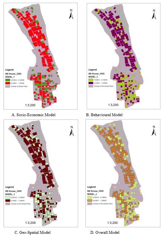
Variations among the Land Plots

Third objective of the research is to quantify the variations in conversion using models. Hence, probability maps of the models in Figure 1 represent variations in each sector as well as the overall variation through the period 2005 (base year in the models) to 2012 in the study area. Therefore, human interactions such as the householders’ behaviour and economic conditions as well as geo-spatial status are the main influences responsible for changing their lands from low-lying plots to home gardens. Another significant fact is that all houses established on low-lying areas have the basic tendency to change their land plots to home garden condition. Each house’s status up to now has been measured for the models. But the process of change will continue because the final goal of every household is to turn its land plot into a home garden to live in.

See Full Size >

Conclusion

In the sectorial models, the important variables / sectors that affect low-lying housing plot conversion have been identified, but it is also important to know the most influential variables. This task is performed using the overall model, the three sectorial models and the validation model. The overall model consists of 19 variables including all variables of the groups except family savings (because of its multicollinearity with family income). The overall model contains 19 variables, out of which 8 variables are significant. The crucial fact is that there are three variables from the geo-spatial group (LLP, GWS & RWR), three variables from the behaviour group (PPG, TSA & PPP) and two variables from the socio-economic group (HI & SKJ) that are significant in the overall model. In the conversion of low-lying land, the strongest variables are the geo-spatial and behaviour variables as they have empirically and statistically demonstrated it. Thus, the overall model has convincingly identified the most important variables that influence the emergence of households on low-lying lands.

Spatial logistic model results have been linked with the spatial database of GIS map so that it indicates the areas converted by establishment of households as well as the non-converted areas. Hence, this classification has been done based on spatial logistic model results. Urban Planning authorities can distinguish between the converted and non-converted areas and even the assessment values of the individual land plots. Therefore, this model can be used as a geo-spatial management system for low lands under threat in other places as well. Thus, the contribution made by this study will be very useful for local government bodies and environmental authorities when they are planning for sustainable development of their urban low lands (Table 04 ).

In this study, all influential factors have been identified and grouped into three key sectors, based on the relevant literature review; the variables in the key categories were then investigated in detail. In the past, several studies devoted to land conversion in low-lying areas have addressed only socio-economic factors. But as a result of the sectorial level analysis conducted by this study, it has been proven that geo-spatial factors (89.5%) and behaviour factors (86.7%) are more influential than the socio-economic factors (81.3%). Therefore, it is now clear that geo-spatial factors and behaviour factors carry at least as much weight as socio-economic factors. Compared to previous studies that did not address all of the above factors in the conversion of low-lying areas, the additional sectorial information that has been included in this study will prove very useful in managing conversion of land and related activities and contribute substantially to future urban planning in low-lying areas.

Acknowledgments

Authors acknowledge the School of Humanities, Universiti Sains Malaysia for the waiver of registration fees for INCoH 2017.

References

1. Arbuckle, J. L. (2010). IBM SPSS Amos 19 user’s guide. Crawfordville. FL:Amos Development Corporation .
2. Chong, I. G., & Jun, C. H. (2005). Performance of some variable selection methods when multicollinearity is present. Chemometrics and Intelligent Laboratory Systems, 78(1), 103-112. https://dx.doi:10.1016/j.chemolab.2004.12.011
3. Dayaratne, R. (2010). Moderating urbanization and managing growth: How can Colombo prevent the emerging chaos? Working paper//World Institute for Development Economics Research. Retrieved from: http://hdl.handle.net/10419/54061
4. Dong, J. J., Tung, Y. H., Chen, C. C., Liao, J. J., & Pan, Y. W. (2011). Logistic regression model for predicting the failure probability of a landslide dam. Engineering Geology, 117(1), 52-61. https://dx.doi:
5. Lee, K. I., & Koval, J. J. (1997) Determination of the best significance level in forward stepwise logistic regression. Communications in Statistics-Simulation and Computation 26, 559-575.
6. Liao, F. H., & Wei, Y. D. (2014) Modeling determinants of urban growth in Dongguan, China: a spatial logistic approach. Stochastic environmental research and risk assessment 28, 801-816. https://doi:
7. Makunde, G. (2016) Challenges in urban development control and housing provision: a case of Epworth, Chitungwiza and Harare, Zimbabwe. International Journal of Technology and Management 1, 1-12.
8. Samat, N. (2007). Integrating GIS and celular automata spatial model in evaluating urban growth: prospects and challenges. Universiti Teknologi Malaysia, Faculty of Built Environment.
9. Samaratunga, T. C., & O'Hare, D. (2013) ‘Sahaspura’: the first high-rise housing project for low-income people in Colombo, Sri Lanka. Australian Planner, 51(3), 230-231.
10. Smith, K. W., & Sasaki, M. S. (1979). Decreasing Multicollinearity A Method for Models with Multiplicative Functions. Sociological Methods & Research, 8(1), 35-56.
11. Vasconcelos, D. M. J .P, Silva, S., Tome, M., Alvim, M., & Pereira, J. M. C. (2001). Spatial prediction of fire ignition probabilities: comparing logistic regression and neural networks. Photogrammetric Engineering and Remote Sensing, 67(1), 73-81.
12. Xie, C., Huang, B., Claramunt, C., & Chandramouli, C. (2005). Spatial logistic regression and gis to model rural-urban land conversion. Paper presented at the Proceedings of PROCESSUS Second International Colloquium on the Behavioural Foundations of Integrated Land-use and Transportation Models: Frameworks, Models and Applications.
13. Zainodin, H. J., Noraini, A., & Yap, S.J. (2011). An alternative multicollinearity approach in solving multiple regression problem. Trends in Applied Sciences Research, 6(11), 1241-1255.