
Study Of The Mechanism Of Increasing Productivity Of Multi-Industry System


Abstract
The article studies a multi-industry system in which industries are active objects. Their activity in this context is manifested in changes in their own technologies in order to maximize profits. This, in turn, affects the coefficients of direct and total material costs. As a result, labor and capital intensity change. A mathematical model has been developed to analyze the patterns of these changes. The production function of the industry as an element of the system is suggested. A mathematical problem is formulated that reflects the industry's desire to maximize profits in the context of intersectoral relations. The solution to the problem is a formula that determines the most acceptable coefficients of direct material costs for the industry as a function of prices. The coefficients of direct material costs affect all parameters of the system, including the coefficients of total labor costs. The latter, according to the labor theory of value, are the basis of prices. To study the results of the mutual influence of cost and price coefficients, a two-level model has been developed. The lower level is represented by models of active industries. The upper level plays the role of a price regulator. The universal regulator is the market. But this function, at least partly, can also be assumed by some macroeconomic regulation body. The model calculation shows that the process quickly converges to a stationary state.
Keywords: Maximization of productivitymulti-Industry systemneoclassical industry modeloptimization of industry interaction
Introduction
In the classical Leontiev model, each industry is represented by only one technology (Leontiev, 1981). The coefficients of direct material costs are constants. In reality, industries are active objects (Miller & Blair, 2009). They restructure technologies according to their own interests and the external situation. This leads to a change in the coefficients of direct material costs. As a result, the entire inter-industry balance changes. It is interesting to consider what the patterns of these changes are and what they lead to.
Problem Statement
Let's form a model of the industry as an element of a multi-industry system. Following the neoclassical theory, we assume that the industry is described by a power production function. Then the gross volume of the industry as a function of the products used by it can be represented as follows: (1)
Where is the scale multiplier; - elasticity, .
Let's divide both parts (1) by :
.
Given that, we get:
. (2)
The set of solutions to this equation is infinite. Of all the possible solutions, the industry will prefer the one that gives it the maximum profit. In this context, it results in maximizing the specific margin income, i.e., in solving the problem
where - the prices of the products.
Research Questions
Let's solve problem (2) and study the solution in the context of intersectoral relations. Let's assume that the prices of the products are known. Let's define the optimal technology as a function of prices. Let's apply the method of Lagrange multipliers.
. (4)
The conditions of stationarity:
Let's use the last equation of the system to express the Lagrange multipliers in terms of the remaining parameters:
Using this expression, we obtain a solution that defines the coefficients of direct material costs as a function of prices:
. (5)
Let's consider the question of prices. Leontiev's model implicitly contains Marx's labor theory of value. Indeed, according to this theory, price is the monetary expression of value, and value reflects the socially necessary costs of labor. In the Leontiev model, this category appears in the form of coefficients of total labor costs (Edinak, 2020).
Let be the number of employees in the i-th industry. By analogy with the coefficients of direct material costs, we introduce the coefficients of direct labor costs: , .
Knowing these coefficients, we can calculate the total demand for labor resources for a given volume of gross output production:
.
Expressing gross production in terms of final production, we write this ratio as follows:
,
where are coefficients of total material costs; is a value that shows how much labor resources of the i-th industry are needed in order to provide with the I-th product the output of a unit of the j-th final product. Summing up for all industries, we get the full labor intensity:
,
It shows how much social labor is needed to produce a unit of the j-th final product. In this case, we will consider these values as the prices of products.
. (6)
Thus, we have found two formulas. Formula (4) shows the dependence of direct cost coefficients on prices, and formula (5) shows the dependence of prices on direct cost coefficients.
Purpose of the Study
The purpose of the study is to find out how the activity of industries associated with increasing their own efficiency affects the entire system. In particular, how the process caused by the mutual influence of costs and prices coefficients affects its productivity. The ratio of total final product to total gross product should be considered an integrated indicator of system productivity (Oosterhaven et al., 2019). The higher this ratio is, the lower the costs of system-wide resources to produce a given final product. The study should answer the question of whether the state of maximum productivity is achievable. If so, what are the conditions for achieving this state. Finally, to what extent the local goals of individual industries coincide with the system-wide goal.
Research Methods
The answers to these questions will be obtained by implementing an iterative process in a two-level model (Figure
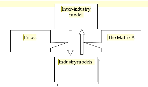
Source: author.
The algorithm is as follows (Figure
1. Perform initial assignments. We assign some initial price values to products, for example , where .
2. Take the next step . Substituting prices in formula (4), we determine the matrix of coefficients of direct material costs .
3. Calculate the current values of the inverse Leontiev matrix, gross product , labor needs .
4. Check the condition where is a sufficiently small number. If the condition is met, stop the process, otherwise go to the next point.
5. Calculate the prices and take them as the initial parameters of the next step. Go to item 2.
6. Output the calculation results.
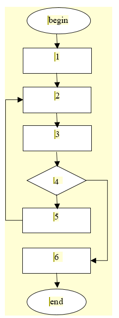
Source: author.
Findings
Let's illustrate the proposed algorithm with a simple example. Let the values of the coefficients of direct material costs, the elasticity of production functions and the coefficients of direct labor costs be given:
.
Let's calculate the matrix in which the product is produced with minimal labor costs. That is, we determine the matrix at which a multi-industry system gives the greatest productivity.
Let's use the original matrix to calculate the scaling factors. It follows from (2) that
.
We get:
Let's assign some initial prices to the products. Let's assume that they are equal to the coefficients of direct labor costs. Next, we will perform a sequence of steps .
The results of the calculation in steps:
As you can see, the process for five iterations converged to a stationary state. Maximum system productivity has been achieved. The initial and final productivity are equal to 0.20 and 0.29, respectively. That is, the productivity of the system increased by 45%.
The study provides a basis for interpreting intersectoral relations in a broader sense than in the classical Leontiev theory. The connection of industries is not limited to the exchange of products. Industries influence each other's production functions. This influence is carried out through the coefficients of direct material costs and prices. Another important conclusion is that the desire of industries to increase their own profits does not contradict the goals of the system. That is, optimization by local criteria leads to the maximum of the general criterion. Price regulation plays an important role in this process (Kichikawa et al., 2020). Achieving system-wide consensus is a condition for maximum productivity. It is expressed in the formation of prices at which no industry seeks to change its technology.
Conclusion
The efficiency of the economy, as a system of interacting industries, depends not only on how effectively individual industries work. It is important how well their technologies, which are reflected in the direct material cost coefficients, are coordinated with each other. If industry technologies do not combine well with each other, then most of the gross product is locked inside the production system. In this case, production largely works for itself. There is an excessive expenditure of labor and other resources. The increase in productivity of a multi-industry system is the result of the laws of the market. But the market mechanism is inertial. Therefore, the mechanisms of macroeconomic regulation play an increasingly important role in the modern economy. The digital economy creates prerequisites for a significant improvement in the quality of such regulation (Shirov, 2018).
References
- Edinak, E.A. (2020). Estimating total labor input for supporting informed economic policy decisions. Studies on Russian Economic Development, 31, 655-662.
- Kichikawa, Y., Iyetomi, H., Aoyama, H., Fujiwara, Y., & Yoshikawa, H. (2020). Interindustry linkages of prices—Analysis of Japan’s deflation. PLoS ONE, 15(2), e0228026.
- Leontiev, A. F. (1981). A generalization of exponential series. Bukinistika.
- Miller, R. E., & Blair, P. D. (2009). Input-output analysis: Foundations and extensions. Cambridge University Press.
- Oosterhaven, J., Polenske, K. R., & Hewings, G. J. D. (2019). Modern regional input-output and impact analysis. In R. Capello, & P. Nijkamp, (Eds.), Handbook of Regional Growth and Development Theories: Revised and Extended Second Edition (pp. 505-525). Edward Elgar Publishing Ltd.
- Shirov, A. A. (2018). Use of input–output approach for supporting decisions in the field of economic policy. Studies on Russian Economic Development, 29, 588-597.
- Shirov, A. A., & Yantovsky, A. A. (2017). Rim cross-industry macroeconomic model - Development of tools in modern economic conditions. Problems of Forecasting, 3, 3-18.
Copyright information

This work is licensed under a Creative Commons Attribution-NonCommercial-NoDerivatives 4.0 International License.
About this article
Publication Date
30 April 2021
Article Doi
eBook ISBN
978-1-80296-105-8
Publisher
European Publisher
Volume
106
Print ISBN (optional)
-
Edition Number
1st Edition
Pages
1-1875
Subjects
Socio-economic development, digital economy, management, public administration
Cite this article as:
Sizikov, A. P. (2021). Study Of The Mechanism Of Increasing Productivity Of Multi-Industry System. In S. I. Ashmarina, V. V. Mantulenko, M. I. Inozemtsev, & E. L. Sidorenko (Eds.), Global Challenges and Prospects of The Modern Economic Development, vol 106. European Proceedings of Social and Behavioural Sciences (pp. 1829-1835). European Publisher. https://doi.org/10.15405/epsbs.2021.04.02.217