
A Bayesian Data Science Approach To A Multilevel Problem In Hrm

Abstract
Data arising in Human Resource Management research usually comes from variables measured at different levels of analysis. These data presents an inherent multilevel structure. Single level models, such as simple or multiple regression, are not suitable for efficient modeling. Hierarchical Linear Models are more appropriate tools, especially if estimated with a Bayesian statistical approach. Three different models have been fitted to a typical multilevel HR data set and compared in a Bayesian setting: a single-level linear model, a two-levels linear model with random intercept and slope, and a cross-level interaction model. The three models have been compared on the basis of the difference in expected log predictive density; The cross-level interaction model was the best one. Reasons for considering the Bayesian framework as the most natural environment for analyzing multilevel data generated in HRM research are outlined. Some advantages, peculiarities, and capabilities of modern software packages designed for Bayesian statistical analysis are also outlined.
Keywords: HRMHLMBayesian analysis
Introduction
Sources of data in Human Resource Management (HRM) are usually placed at several different levels: firm, organization, unit, team, and individual. Employee’s behaviour may be affected by both personal attitudes and organization variables. This is why research in this area asks for parametric models with more than one level (Ostroff & Bowen, 2000; Shen, Messersmith, & Jiang, 2018). Due to the multilevel nature of data structure, single level linear modelling (simple or multiple classical regression) is not suited for exploration, modelling, and prediction of data arising in HRM (Aguinis, Gottfredson, & Culpepper, 2013; Shen et al., 2018; Shen, 2016). When conducting research that includes variables measured at different levels of analysis, researchers explicitly recognize that lower-level entities, such as individuals, are nested within higher-level collectives such as teams (Aguinis et al., 2013). The multilevel nature of data requires dependence among observations to be considered both conceptually and analytically (Snijders & Bosker, 2012). A higher-level variable may covary with relevant lower-level outcomes variables, and entities within collectives may be more similar regarding certain variables compared to entities across collectives (Bliese & Hanges, 2004). It may also happen that the nature of the relationship between lower-level variables depends on higher-level ones, the so-called
HLM in social and behavioural sciences, as well as in HRM, are more often estimated in the frequentist statistical framework (Aguinis et al., 2013; Cohen, Cohen, West, & Aiken, 2003; Muth, Oravecz, & Gabry, 2018). However a Bayesian statistical approach to HLM fitting, besides being the most natural, offers several advantages, in terms of interpretability of estimates and flexibility to increasingly complex models (Muth et al., 2018; Korner-Nievergelt et al., 2015; McElreath, 2016). Until fairly recently, due to computational limitations, practical Bayesian statistical analysis was limited to few applications. Markov-Chain Monte Carlo (MCMC) methods, a suite of random-sampling simulation methods originally formulated in the 1950s in statistical physics, has greatly expanded the application of Bayesian methods to applied data analysis (Fox & Weisberg, 2019; Gelman et al., 2013; Kruschke, 2015). Bayesian modelling has become increasingly accessible and efficient thanks to advances in statistical software and generic estimation engines such as Stan (Stan Development Team, 2017; Carpenter et al., 2017; Kruschke, 2015). Stan implements a species of MCMC methods, called Hamiltonian Monte Carlo, which provides advantages of robustness and efficiency relative to older MCMC methods such as the Metropolis-Hastings algorithm and the Gibbs sampler (Fox & Weisberg, 2019). Several modern Stan-based R packages make some Stan’s functionality available using programming techniques familiar to R users. In this paper we have taken advantage of using the rstanarm R package (Stan Development Team, 2017; Carpenter et al., 2017) that make Bayesian model specification more easy and succinct by miming the syntax of several R’s functions very popular in the frequentist statistical community.
It is well known that, among operative functions of modern HRM, improvement of employees’ relations, team building and leadership management, play a crucial role. As a result of the widespread move to team-based organizations in industry, managers are often asked to lead and motivate both individuals and teams as a whole. When building and fitting statistical models, researchers in this field should consider the dynamic interplay between the individuals within a team and the team as a whole (Chen, Kirkman, Kanfer, Allen, & Rosen, 2007).
In this paper we have considered a typical HR data set concerning individuals grouped in several teams. The data set presents a natural nested (hierarchical) structure and was originated and analyzed in Aguinis et al. (2013). The data set considered in that paper, was patterned after Chen et al. (2007). Among other concepts, several multilevel models were fitted to the data and compared, but in a frequentist statistical setting. However multilevel models naturally fit into the Bayesian paradigm (Kruschke, 2015; Shen et al., 2018; Gelman et al., 2013). This is the reason, in addition to various advantages, for which we have analysed the same data in a Bayesian statistical framework. One single-level linear model, one two-level hierarchical linear model and one cross-interaction two-level linear model have been fitted and compared. General advantages of a modern Bayesian statistical approach, in terms of interpretability of the results, and of modern analytical and graphical tools have been outlined. For the computational aspect of this paper we have taken advantage of the Stan software (Stan Development Team, 2017) and of the R statistical software and some of its packages (R Core Team, 2018).
Literature Review and Theoretical Framework
In this section we presents a review of literature on multilevel modelling in HRM research, on modern Bayesian statistical analysis, and on software availability.
Literature review
For a state of art, wide and exhaustive introduction to multilevel thinking and modelling in HRM research, we refer to Bliese (2002), Renkema, Meijerink and Bondarouk (2017), Shen et al; (2018), Shen (2016), Aguinis et al; (2013), and the references therein. Gelman and Hill (2007) is a good, perhaps dated from a computational point of view, introduction to general Bayesian statistical methods. Gelman et al. (2013) is a quite complete, but mathematically and technically demanding, presentation of modern Bayesian methods with an appendix on using Stan and R. McElreath (2016) is a gentle introduction to Bayesian methods, including multilevel linear models, with R and Stan. Fox and Weisberg (2019) is a good reference for applied regression with R, including multilevel (mixed) models, with a freely available web appendix on Bayesian estimation with Stan. For the Stan program, the state of art in Bayesian statistical software, we manly refer to Carpenter et al; (2017). Gabry and Goodrich (2018) present the rstanarm package, a Stan based R package. Gabry, Mahr, Bürkner, Modrák, and Barret (2018) is the reference for the bayesplot package for plotting Bayesian models. Muth et al. (2018) is an excellent introduction to Bayesian hierarchical linear models fitting with rstanarm package and the user-friendly exploration of results with the shinystan package. References therein can guide the interested readers towards a deeper knowledge of the subject.
The Bayesian approach to model fitting with Stan and rstanarm.
The statistical models presented later in this paper can all be estimated and fitted to data with a frequentist approach. However when data presenting a multilevel structure asks for hierarchical modelling, the Bayesian statistical approach is the most suitable one. The starting point of Bayesian statistics is Bayes’ theorem. In a regression model setting its general form states that the posterior probability distribution of parameters given data and is proportional to the product of the likelihood function, , of the observed response data given the parameters and the regressor data , and the prior distribution of the parameters:
Here we have assumed that, as it is the case in standard regression setting, and are independent, so that the prior doesn’t depend on the regressor .
The most compelling applications of Bayesian methods typically aren't to standard regression models, such as the normal linear model or generalized linear models, but to problem where we want to specify a customized probability model for the data such as a Hierarchical Linear Model, in short HLM (Fox & Weisberg, 2019; Muth et al;, 2018). HLM is an extension of the classical linear model that is well suited for data like ours that present a nested structure where individuals are grouped in teams. Relationships are expected to be similar in the same group and groups are not generally exchangeable (Gelman & Hill, 2007; Hox, Moerbeek, & van de Schoot, 2018). Modeling in the Bayesian statistical framework is mainly composed of four key steps (Muth et al., 2018): data model and prior specification, parameters estimation, sampling quality and model fit checking, results summarization and interpretation. Here, because of space limitations, we will not deeply explore all the four steps. The Stan estimation engine has been used to fit the statistical models described in the next sections via the rstanarm package. We used the default weakly informative priors of rstanarm. The rstanarm package allows the user to easily specify the models considered (Carpenter et al., 2017). Several fundamental tools for MCMC diagnostic are also implemented in the package as well as useful numerical device for results summarization. Graphical representation tools used in this paper are provided by the bayesplot package (Gabry et al., 2018).
We encourage the reader to further explore the literature on Bayesian methods, for example via Gelman and Hill (2007), Gelman et al. (2013), Kruschke (2015), McElreath (2016).
Research Method
In this section we present the data and the statistical models to be fitted to them.
The data
Our data set is part of a publicly available larger data set originated by Aguinis et al., (2013) and patterned after a study by Chen et al; (2007), composed of individual observations of several variables on 630 employee. We have selected 4 columns from the original data set, named as: quality of
The statistical models
The first model considered in this paper is a simple linear model explaining the relationship between the level-1 variables
We will refer to this model as
The second considered model, referred as
This model improves
The third model,
This is the model considered in
For more information about models as
The software
We have intensively used the Stan program (Carpenter et al., 2017) via the rstanarm package (Gabry & Goodrich, 2018), which provides an R software interface to Stan programming. The bayesplot R package (Gabry et al., 2018) has complemented the rstanarm tools providing an extensive library of function for plotting posterior draws, visual MCMC diagnostic, as well as graphical posterior predictive checking.
Findings
In this section we present part of the outputs of the Bayesian analysis aimed to fit models to data. Results for different models are in different subsections.
Results for model1 fitting.
The estimated posterior mean, standard deviation and 95% Credible Intervals (CI’s) for the intercept b0, the slope b1 and the residual standard error s for
Results for model2 fitting.
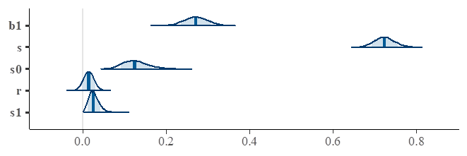
Results for
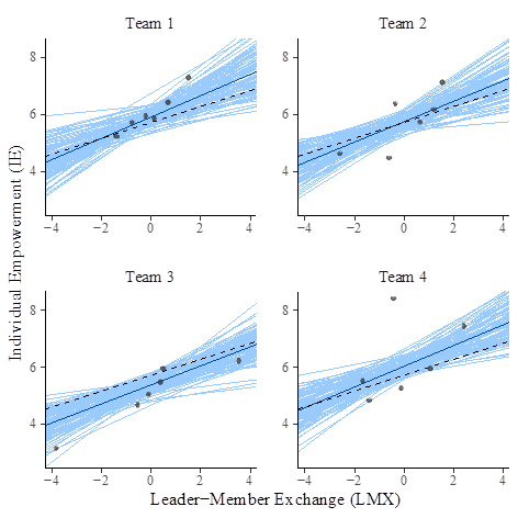
In Figure
In Figure
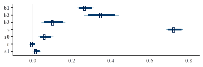
Results for model3 fitting.
Results for
Results of a more analytic model comparison are presented in the next subsection.
Model comparison.
We have evaluated our models with the leave-one-out (loo) cross-validation and compared them on the basis of the difference in expected log predictive density (
Conclusion and Discussions
Research in HRM is inherently a multilevel field of study as data originated in this field usually has an intrinsic hierarchical structure. Although until a few years ago HRM research has been conducted only at the single level of analysis, single level statistical tools, such as linear model, are not ideal. Multilevel modelling was first used in education and marketing research (Shen et al., 2018). Very recent trends have witnessed a growing use of hierarchical linear model (HLM) in HR literature, but estimation efforts of these models are more often faced with a frequentist statistical approach. The Bayesian statistical approach is actually ideally suited for constructing hierarchical models, and it is therefore very useful for analysing data structures with multiple levels, such as data from individuals who are members of groups which in turn are in higher-level organizations (Kruschke, 2015; Kruschke & Vanpaemel, 2015; Gelman et al;, 2013).
In this study we have fitted in a Bayesian statistical framework three different models to a data set originated and analyzed in Aguinis et al; (2013) with a frequentist approach. The goal of that paper was to investigate whether the quality of
Although the majority of HRM research has historically been conducted at the single level of analysis (Shen, 2016), today it is well known that multilevel modelling significantly advances HRM research by more accurately predicting HRM effects and estimating complex HRM models (Shen et al;, 2018). In this paper we have shown, with a concrete example, how modern computational, diagnostic and representation tools have made the Bayesian statistical approach the most convenient as well as the most natural paradigm for analysis and modelling of multilevel data arising in HRM research.
References
- Aguinis, H., Gottfredson, R. K., & Culpepper, S. A. (2013). Best-practice recommendations for estimating cross-level interaction effects using multilevel modeling. Journal of Management, 39(6), 1490-1528.
- Bliese, P. D. (2002). Multilevel random coefficient modeling in organizational research: Examples using SAS and S-PLUS. In F. Drasgow & N. Schmitt (Eds.), Measuring and analyzing behavior in organizations: Advances in measurement and data analysis: 401-445. San Francisco: Jossey-Bass.
- Bliese, P. D., & Hanges, P. J. (2004). Being both too liberal and too conservative: The perils of treating grouped data as though they were independent. Organizational Research Methods, 7, 400-417.
- Carpenter, B., Gelman, A., Hoffman, M., Lee, D., Goodrich, B., Betancourt, M., …& Riddell, A. (2017). Stan: A probabilistic programming language. Journal of Statistical Software, Article, 76(1), 1-32.
- Chen, G., Kirkman, B. L., Kanfer, R., Allen, D., & Rosen, B. (2007). A multilevel study of leadership, empowerment, and performance in teams. Journal of Applied Psychology, 92, 331-346.
- Cohen, J., Cohen, P., West, S. G., & Aiken, L. S. (2003). Applied multiple regression/correlation analysis for the behavioral sciences. Routledge.
- Fox, J., & Weisberg, S. (2019). An R Companion to Applied Regression. Sage, Thousand Oaks, CA, third edition.
- Gabry, J., & Goodrich, B. (2018). Rstanarm: Bayesian Applied Regression Modeling via Stan. R package version 2.17.4. http://mc.stan.org/rstanarm
- Gabry, J., Mahr, T., Bürkner, P. C., Modrák, M., & Barret, M. (2018). Bayesplot: plotting for Bayesian models. R package version 1.6.0. Retrieved from http://mc-stan.org/bayesplot
- Gelman, A., Carlin, J. B., Stern, H. S., Dunson, D. B., Vehtari, A., & Rubin, D. B. (2013). Bayesian data analysis, Third edition. Boca Raton (FL): Chapman & Hall/CRC.
- Gelman, A., & Hill, J. (2007). Data analysis using regression and multilevel/hierarchical models. Cambridge: Cambridge University Press.
- Hox, J. J., Moerbeek, M., & van de Schoot, R. (2018). Multilevel Analysis. Techniques and Applications. New York, NY: Routledge.
- Korner-Nievergelt, F., Roth, T., von Felten, S., Guélat, J., Almasi, B., & Korner-Nievergelt, P. (2015). Bayesian data analysis in ecology using linear models with R, BUGS, and Stan. Academic Press.
- Kruschke, J. K. (2015). Doing Bayesian data analysis: A tutorial with R, JAGS, and Stan. Academic Press.
- Kruschke, J. K., & Vanpaemel, W. (2015). Bayesian estimation in hierarchical models. In: J. R. Busemeyer, Z. Wang, J. T. Townsend, & A. Eidels (Eds.), The Oxford Handbook of Computational and Mathematical Psychology, pp. 279-299. Oxford, UK: Oxford University Press.
- McElreath, R. (2016). Statistical rethinking: a Bayesian course with examples in R and Stan. CRC Press.
- Muth, C., Oravecz, Z., & Gabry, J. (2018). User-friendly Bayesian regression modeling: A tutorial with rstanarm and shinystan. The Quantitative Methods for Psychology, 14(2), 99-119. https://dx.doi.org/1020982/tqmp.14.2.p099
- Ostroff, C., & Bowen, D. E. (2000). Moving HR to a higher level: HR practices and organizational effectiveness. In K. L. Klein, & W. J. Kozlowski (Eds.), Multilevel theory, research, and methods in organizations: Foundations, extensions, and new directions (pp. 211-266). San Francisco, CA: Jossey-Bass.
- R Core Team (2018). R: A language and environment for statistical computing. R Foundation for Statistical Computing, Vienna, Austria. Retrieved from https://www.r-project.org
- Renkema, M., Meijerink, J., & Bondarouk, T. (2017). Advancing multilevel thinking in human resource management research: Application and guidelines. Human Resource Management Review, 27(3), 397-415.
- Shen, J. (2016). Multilevel analysis in HRM research using HLM: Principle and application. Human Resource Management, 55, 951-965.
- Shen, J., Messersmith, J. G., & Jiang, K. (2018). Advancing human resource management scholarship through multilevel modeling. The International Journal of Human Resource Management, 29(2), 227-238.
- Snijders, T. A., & Bosker, R. J. (2012). Multilevel Analysis: An introduction to basic and advanced multilevel modeling, 2nd ed.. Los Angeles, CA: Sage.
- Stan Development Team. (2017). Stan modeling language users guide and reference manual, version 2.17.0. Retrieved from http://mc-stan.org/
- Vehtari, A., Gelman, A., & Gabry, J. (2017). Practical Bayesian model evaluation using leave-one-out cross-validation and WAIC. Statistics and Computing, 27(5), 1413-1432.
Copyright information

This work is licensed under a Creative Commons Attribution-NonCommercial-NoDerivatives 4.0 International License.
About this article
Publication Date
30 October 2019
Article Doi
eBook ISBN
978-1-80296-070-9
Publisher
Future Academy
Volume
71
Print ISBN (optional)
-
Edition Number
1st Edition
Pages
1-460
Subjects
Business, innovation, Strategic management, Leadership, Technology, Sustainability
Cite this article as:
Giosa*, M. D. (2019). A Bayesian Data Science Approach To A Multilevel Problem In Hrm. In M. Özşahin (Ed.), Strategic Management in an International Environment: The New Challenges for International Business and Logistics in the Age of Industry 4.0, vol 71. European Proceedings of Social and Behavioural Sciences (pp. 208-218). Future Academy. https://doi.org/10.15405/epsbs.2019.10.02.19