
Developing A Simulation System For Modelling The Product Life Cycle Using Anylogic


Abstract
The article considers the relevance of simulation modelling of various situations in the modern world, describes modelling methods and analyses the subject area, which is the product life cycle and its curves. The AnyLogic environment is chosen to develop a system for simulating the consumer market and charting the product life cycle. The article describes the course of development, consumer specific states and the factors affecting them, sets the interaction mechanism, and at the end gives the system results. Modern world is impossible to exist without modelling various situations (economic, political, social or others), which often plays an important role in risk assessing and forecasting a particular business or enterprise development. Each product exists on the market for a certain time and then sooner or later it is replaced by another, more perfect one. In this regard, the concept of the product life cycle is introduced. The concept of the product life cycle describes the stages of any product or service development, from the moment it first appears on the market to its sale termination and production end.
Keywords: AnyLogic, expert systems, life cycle, modelling, simulation modelling
Introduction
Simulation models provide an opportunity to test various ideas, hypotheses and assumptions regarding an enterprise development or a business strategy implementation, and analyse their fulfilment consequences. The enterprise activity in the model is reproduced, for instance, by describing the cash flow movement as events occurring in different periods of time, operations within the enterprise and the input or external data affecting its work (Filippov et al., 2020). With the help of models, one can play various behaviour scenarios of consumers, suppliers, competitors, which largely determines an enterprise development in the future.
Problem Statement
The classic product life cycle curve looks like a graph of sales and profits over time. Figure 1 shows the main stages of the product life cycle: market introduction stage, growth stage, product maturity stage, sales decline stage.
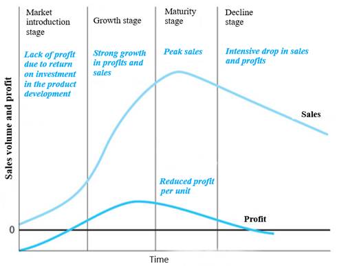
“The market introduction stage” is characterized by low sales, low growth, and relatively high investment to support the product. The length of the period depends on the intensity of the company’s efforts to distribute the product on the market (Lychkina, 2005).
“The growth stage” is the most important stage in the product life cycle. At that stage, the future success of the new product is laid. The growth phase is characterized by high sales and increased profits, which can now be reinvested in programmes to develop the new product (Karpov, 2005; Kelton & Lou, 2004). At the growth stage, the first competitors appear who borrow successful production technology and product quality.
In “the product maturity stage”, the product reaches its maturity, sales and profit levels stabilize, and growth slows down. The product becomes sufficiently known in the market and can exist with the minimal support.
“The sales decline stage” is characterized by a significant decrease in sales and profits. Consumers are beginning to abandon the product in favour of more modern, new and technological innovations in the market. But despite the decline in demand, the company still has loyal conservative consumers.
Research Questions
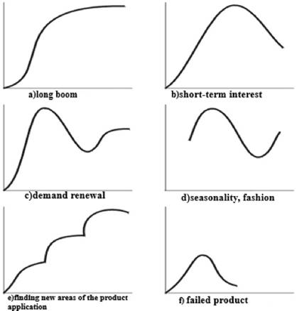
Despite the popularity of the product life cycle theory, there is no evidence to support that most products go through a typical four-phase cycle and have standard life cycle curves (Emelyanov et al., 2002). There is also no evidence that the turning points of the various phases of the life cycle are more or less predictable. In addition, different types of life cycle curves can be considered depending on the level of aggregation at which the product is considered (Figure 2).
In this case, if it is necessary to predict the results of a new product entering the market, its profit or, conversely, the loss and costs, one can use simulation modelling and build a system simulating the work of the market and consumers, and make a product life cycle chart for the given initial values.
Purpose of the Study
Simulation modelling is developing and executing a software system on a computer that reflects the structure and functioning or behaviour of a simulated object or phenomenon in time. A simulation model is a simplified version of a real system, either an existing one or one that is supposed to be created in the future. The simulation model is usually represented by a computer programme, the execution of which can be considered an imitation of the original system behaviour in time (Efromeeva, 2020).
Simulation modelling has significant advantages over analytical modelling when:
- the relationships between the variables in the model are not linear and therefore analytical models are difficult or impossible to construct;
- the model contains stochastic components;
- it is required visualizing the dynamics of the processes taking place in it to understand the system behaviour;
- the model contains many parallel functioning interacting components.
In many cases, simulation is the only way to understand and analyse the complex system behaviour.
Simulation modelling is implemented through a set of mathematical tools, special computer programmes and techniques that allow using a computer to conduct targeted modelling in the “simulation” mode of the complex process structure and functions and optimize some of its parameters. A set of software tools and modelling techniques determines the specifics of the modelling system, namely special software.
Unlike other types and methods of mathematical modelling using computers, simulation modelling has its own specifics such as the launch of interacting computational processes in a computer, which are analogues of the processes under study in terms of their timing parameters up to time and space scales.
There are a number of simulation systems:
- CHEMCAD software package.
- Design II for modelling in oil and gas processing.
- Software for simulating technological processes PRO/II.
- ProMax for designing and optimizing gas processing, oil processing and chemical industries.
- The GIBBS software product has tools for modelling the field preparation of natural gases.
- Simulation system “Comfort” for verification and design calculations of material and heat balances of various chemical industries.
- Others.
For developing the simulation system described in this article, AnyLogic is used due to a number of advantages examined below.
Research Methods
Statement of the Problem
The current part of the article describes the stages of building an agent-based model that will help to study the process of bringing a new product to the market, consumption and decommissioning.
During the development process, the following tasks are to be solved:
- To consider a relatively small consumer market of 5,000 people.
- To analyse the process of bringing to the market a new product, which initially no one uses and people will start buying the product under the advertising impact. After this initial stage, sales will be much more influenced by people talking to each other, recommendations and positive feedback from the product consumers, encouraging others to purchase it.
- To determine the service life and delivery time, as well as the time of using the product and the consumer expectations. All these factors will imitate agents’ behaviour as buyers, who will become new buyers from potential customers under various factors and after decommissioning the product may purchase it again.
- To display on the diagram the demand for the product and the market saturation. To add sliders to vary the input data and display the agents-buyers’ population for clarity.
Creating a Population of Agents
At the beginning, the Market model is created. To implement consumers in it, one needs to create a large number of agents of the same type; therefore, using the “Agent Creation Wizard”, the “Agent Population” option is selected. A population of agents “Consumers” is created, with a dimension of 5000 people. Each agent living in the created population will simulate a separate consumer agent. To display a population unit, the output animation of a two-dimensional sprite model is configured. In “Build Environment Configuration”, the option “Apply Random Location” is selected to place agents randomly in space (Filippov et al., 2016).
The environment specifies the type of space in which agents live, agents’ location, and the network of agents’ contacts that can be used when they communicate with each other.
Using the property “Spaces and Network” of the base agent Main, the environment settings for the created population are changed namely the environment width and length and the agents’ location type.
Among agent Main’s properties “Specific”, the option “Draw the agent with a shift from a given point” is selected. Thus, the population animation figure sets the upper left corner of the rectangle, inside which the animation figures of the population agents will be located during the model execution (Kuz'menko & Kondrashin, 2019).
If you run the model at this stage, the model window will appear. You can see the model presentation which is 5000 agents’ animation figures of the consumer population. Since at this stage the rules for the agent’s behaviour are not set, nothing else happens on the animation.
Specifying the Consumer Behaviour
The agent’s behaviour within the framework of this simulation model will be presented as follows: it is assumed that each of the agents has several characteristics, these are:
- “Advertising Effectiveness” (AdEffectivness) is percentage of the potential consumers who want to buy a product during the day due to exposure to advertising. Value = 0.004 is selected for the model.
- “Contact Rate” (ContactRate) is the number of meetings per day with other agents. For the model, the value = 1 person per day is selected.
- “Purchase probability” (AdortionFraction) is the probability of purchasing a product by a potential consumer under the influence of communication with another agent. The value = 0.01 is chosen for the model.
- “Operating time of the goods by the buyer” (DiscardTime) is the time during which the goods will be out of service. Let us assume that the product in question has a limited shelf life (or useful life) of six months.
For the Consumer agent population, the corresponding parameters are set with the given initial values.
These characteristics affect the agent’s state, such as:
- “Potential Buyer” (Potential User) is an agent who has not bought or does not use the goods.
- “Wanting to buy (Waiting for goods)” (WantsToBuy) is an agent who has placed an order, a waiting consumer.
- “Consumer” (User) is the agent who has received and uses the goods.
The following describes the agents’ behaviour using a state diagram.
State diagrams (state maps, statecharts) are the most convenient means of specifying the agent’s behaviour. Statecharts contain states and transitions. The diagram states are mutually exclusive, that is, an agent can only be in one state at a time. Firing a transition leads to changing a state and activating new transitions. It is allowed to create hierarchical states that contain other states and transitions inside. One agent can have several state diagrams at once, each of which describes independent aspects of the agent’s behaviour (Leonov et al., 2018).
Drawing a statechart always starts by adding the beginning of the statechart. And then the first initial state of the agent is connected to it.
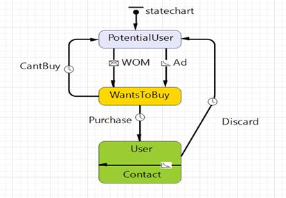
The relationships between these states will be described by the following state transitions:
Advertising (Ad) is the transition from the Potential User state to the User state, simulating how a person acquires a product (and becomes its consumer).
In the transition property “Occurs” the option “With a given intensity” is chosen. In the “Intensity” field, the name of the variable Ad Effectiveness is set as a trigger for the transition to the next state.
Contact (Contact) is a cyclic transition within the User state, occurring with a given intensity equal to the value of the Contact Rate parameter. Each time this transition fires, the called function sendToRandom(“Buy”) simulates this consumer sending a “Buy” message to a randomly selected agent. If the agent receiving the message is a potential consumer (that is, in the Potential User state), then the current state of the receiving agent will be the User state (according to another transition, which is described below).
WOM is the transition from the Potential User state to the User state, simulating the purchase of a product as a result of other people’s recommendations.
In the “Occurs” list, “When receiving a message” is selected. In the “Make the transition” property, “On receiving the specified message" is selected. The “Message” field says “Buy”. Since not every contact leads to new sales, a limit on the proportion of successful contacts has been introduced using the Adoption Fraction parameter applying an additional transition condition: randomTrue (AdoptionFraction)
Discard is a transition triggered by a timeout equal to the value of the DiscardTime parameter
Purchase is the transition from the WantsToBuy state to the User state to simulate the delivery and, accordingly, the purchase of goods.
The fact is taken into consideration that the time consumers agree to spend waiting for the delivery of goods tends to be minimal. If the delivery time exceeds the maximum allowable waiting time, the consumer will abandon the purchase. To simulate this situation, let’s introduce on the Main diagram two parameters that specify the maximum delivery time of the goods (25 days) and the maximum delivery waiting time (7 days), respectively.
The MaxWaitingTime parameter specifies the maximum time during which the consumer is ready to wait for the product delivery (in our case, 7 days). Another parameter, MaxDeliveryTime, sets the maximum possible delivery time for the goods (in our case, 25 days).
The delivery time value from a fixed period of two days is then replaced with a stochastic expression that uses the above range of values applying the AnyLogic probability distribution. The triangular (1, 25, 2) expression will be automatically inserted into the timeout value field, which is manually corrected to the expression triangular (1, main.MaxDeliveryTime, 2) .
CantWait is a transition that leaves the WantsToBuy state and leads to the Potential User state. This transition simulates how the consumer refuses to buy a product due to its long absence.
As a result, the state diagram of the Consumer agent will look like this (Figure 3).
Charting
One needs to know visually how many people purchased the product at a certain point in time. For this, functions are set that will count the number of consumers who want to buy the product and potential consumers, respectively, and then a chart is added to observe the dynamics of the market change.
To display the statistics data, the “Stacked timing chart” is used.
To set what data the graph will display, we will use the same statistics functions created earlier for the Consumers population and set the following chart settings.
Control Customization
Models can be made interactive by adding various controls (buttons, sliders, text fields, etc.) to the model interface. The controls can be used both to set parameter values before starting the model execution, and to change the model right in its execution course. Controls that have state or contents (such as a slider, a radio button, a text box, etc.) have a current value and can be associated with variables and settings so that when the user changes the state of that control, the value of the element associated with it also changes (but not vice versa).
In addition, one can set a specific action for the control, such as calling a function, scheduling an event, sending a message, stopping the model, and so on. The action will be executed every time the user changes the control state.
Sliders have been added to this model; a slider is a control element that allows selecting a numeric value from a certain interval. The slider is often used to change the values of numerical variables and parameters.
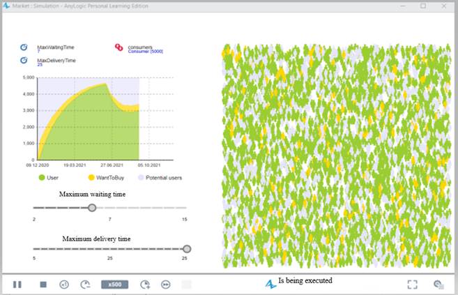
By changing the maximum waiting time and the maximum delivery time using the sliders, one can evaluate the impact of these changes on consumer behaviour and market conditions. The results of the work done and the finished model are shown in Figure 4.
All figures and tables should be referred in the text and numbered in the order in which they are mentioned.
Findings
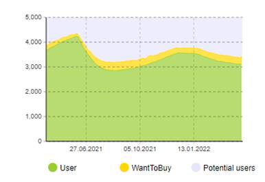
With the given system parameters, we get the PLC curve (Figures 5-6), close to the classical curve. Rapid growth in sales of about 4500 units, short-term maturity, and a gradual decline are clearly visible. Further, during the simulation, the chart shows how the graph goes up slightly and falls again until it turns into an almost straight line, which indicates the support of the life cycle by regular consumers.
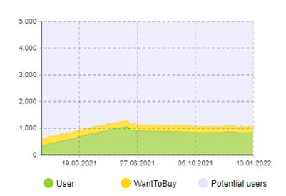
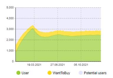
By setting new input data using controls or changing the agent settings, one can get different results: for example, by reducing the exposure of the consumer to advertising and the number of days he waits the graph will look flat, and sales will be low (Figure 7), while by reducing the product service life and increasing the probability of buying after the recommendation considering that saturation with the goods will occur when 3,000 units are sold, the chart will demonstrate a short-term increase and then weak sales.
Conclusion
As a result of building a simulation model of the product life cycle, a chart of the product life cycle is created with the given initial values. It should be concluded that if the product life cycle is very long, there is saturation with this product in this market. If the life cycle becomes no longer time-consuming, there is a complete saturation with goods. So, if the product life cycle is still very short, there is a shortage of this product in the consumer market. Hence, it is always necessary to select the optimal terms for the product life cycle by varying the data.
References
Efromeeva, E. V. (2020). Imitacionnoe modelirovanie: osnovy prakticheskogo primeneniya v srede anylogic. Uchebnoe posobie [Simulation modeling: fundamentals of practical application in AnyLogic. Textbook]. University education. DOI:
Emelyanov, A. A., Vlasova, E. A., & Duma, R. V. (2002). Imitacionnoe modelirovanie ekonomicheskih processov [Simulation Modelling of Economic Processes]. Finance and Statistics, 368. https://institutiones.com/download/books/1761-imitacionnoe-modelirovanie-ekonomicheskix-processov.html
Filippov, R. A., Filippova, L. B., & Sazonova, A. S. (2016). Internet veshchej: osnovnye ponyatiya [Internet veshchey: osnovnyye ponyatiya]. Publishing house of BSTU. Text: electronic. Russian State Library: [website]. Retrieved on 07 June, 2022 from https://search.rsl.ru/ru/record/01008894495
Filippov, R. A., Kuzmenko, A. A., Filippova, L.B., & Sazonova, A.S. (2020). Intelligent System of Classification and Clusterization of Environmental Media for Economic Systems. Proceedings of the International Conference on Economics, Management and Technologies 2020 (ICEMT 2020). - Advances in Economics, Business and Management Research, 139, 583-586. DOI:
Karpov, Yu. (2005). Imitacionnoe modelirovanie sistem. Vvedenie v modelirovanie s AnyLogic 5. [Introduction in Modelling and Simulation with AnyLogic 5]. BHV-Petersburg. Book guide [website]. Retrieved on 02 June, 2022 from https://knigogid.ru/books/122662-imitacionnoe-modelirovanie-sistem-vvedenie-v-modelirovanie-s-anylogic-5
Kelton, V. D., & Lou, A. M. (2004). Simulation modelling. Classic CS. (3rd Ed.) BHV Publishing Group.
Kuzmenko, A. A., & Kondrashin, D. Ye. (2019). Metody i podhody k razrabotke sistemy avtomatizirovannogo analiza dinamiki izmeneniya ploshchadi lesnyh nasazhdenij na osnove metodov avtomaticheskogo raspoznavaniya obrazov [Methods and approaches to the development of a automated analysis’s system of the changes’ dynamics in the area of forest plantations based on the methods of automatic pattern recognition]. ERGODIZAYN, 4(6). https://www.doi.org/
Leonov, E. A., Leonov, Y. A., Kazakov, Y. M., & Filippova, L. B. (2018). Intellectual Subsystems for Collecting Information from the Internet to Create Knowledge Bases for Self-Learning Systems. Proceedings of the Second International Scientific Conference “Intelligent Information Technologies for Industry” (IITI’17). IITI 2017. Advances in Intelligent Systems and Computing), 679. Springer International Publishing. https://www.springerprofessional.de/en/intellectual-subsystems-for-collecting-information-from-the-inte/15096932
Lychkina, N. N. (2005). Imitacionnoe modelirovanie ekonomicheskih processov [Simulation model for economic processes]. IT Academy. http://simulation.su/uploads/files/default/2005-uch-posob-lychkina-1.pdf
Copyright information

This work is licensed under a Creative Commons Attribution-NonCommercial-NoDerivatives 4.0 International License.
About this article
Publication Date
29 August 2022
Article Doi
eBook ISBN
978-1-80296-126-3
Publisher
European Publisher
Volume
127
Print ISBN (optional)
-
Edition Number
1st Edition
Pages
1-496
Subjects
Economics, social trends, sustainability, modern society, behavioural sciences, education
Cite this article as:
Kuzmenko, A. A., Filippova, L. B., & Sazonova, A. S. (2022). Developing A Simulation System For Modelling The Product Life Cycle Using Anylogic. In I. Kovalev, & A. Voroshilova (Eds.), Economic and Social Trends for Sustainability of Modern Society (ICEST-III 2022), vol 127. European Proceedings of Social and Behavioural Sciences (pp. 457-467). European Publisher. https://doi.org/10.15405/epsbs.2022.08.50