The Management Process Construction In A Multifactorial Economic System

Abstract

The problem of constructing the process of managing the economic system with the possibility of taking into account an arbitrary finite number of factors influencing its development is solved. The criterion for improving the well-being of the population against the background of sustainable economic growth was adopted as an optimization criterion. In the formulation of the problem, indicators are introduced that take into account the level of specific efficiency of investments in the corresponding factors of development of the economic system. An algorithm for the optimal distribution of investments is proposed that maximizes the optimization criterion over a given time interval. The solution to the optimal planning problem is found using a combination of analytical and numerical methods. The developed method for constructing the process of managing the economic system, taking into account an arbitrary number of factors, has a practical application. It can be used in constructing strategies and management in regional socio-economic systems.

Keywords: Mathematical modeling, economic system, factors, process of managing, maximum principle

Introduction

The process of functioning of economic systems is the movement of financial, material and information flows that form the manufactured product. Expressed in monetary form, it is divided into parts: investments in production activities, in the social sphere, in increasing production efficiency, etc. The distribution should be carried out in an optimal way, based on the criteria for increasing the efficiency of the economy, taking into account the limited sources of additional investment and the need to increase the investment attractiveness of the region.

The construction of strategies for the optimal allocation of funds belongs to the class of control problems. A special place among the tasks of optimal management of economic systems is occupied by tasks, the solution of which is development strategies with the aim of increasing the welfare of the population against the background of sustainable economic growth. The solution of such problems is presented, for example, in the works Alonso-Carrera et al. (2021), Ketova et al. (2013), Ketova and Saburova (2020).

In many practical applications, when constructing a strategy for optimal control of economic systems, a one-factor macromodel of economic dynamics is used, known as the Ramsey-Kass-Koopmans model Ramsey (1928), Cass (1965), Koopmans (1965), the development of which is presented by the works of Makarov V., Rubinov A., Belenky V., Matveenko V. This is described in the monograph Belenkii (2016). Most of the works consider one-factor models or, less often, two-factor models. So, single-product dynamic models for studying the influence of the gross product on the formation of regional financial potential are used in the work of Davydenko et al. (2021), to build optimal management in a single-industry economy – in the work of Grigorenko and Luk’yanova (2021), the work of Agarkov and Tarasyeva (2020) studied the proportional development of the economic system based on a one-factor macromodel of the economy. In the work of Ren et al. (2021), a two-factor model is used to analyze statistical information and to build effective management in a model of economic dynamics. The work of Kiselev et al. (2020) presents the results of mathematical analysis and numerical experiments of a two-sector economy.

In most cases, multifactorial problems are solved by reducing them to one-factorial ones. A method for moving from a multidimensional to one-dimensional problem setting is given in Esfandiari (2020) and Belenkii and Ketova (2006).

The development of a mathematical apparatus for solving problems with an arbitrary number of factors makes it possible to consider a wider range of applied problems. A group analysis of problems that can be formulated on the basis of classical models of economic dynamics is given in the work of Polat and Ozer (2020).

A distinctive feature of the problem formulation for the economic system management in this work is the ability to take into account an arbitrary number of economic development factors. The proposed model is designed to carry out predictive scientific and analytical calculations of economic development; the results of experimental calculations in the case of a two-dimensional model are presented on the example of the Udmurt Republic.

The result of solving the control problem is the optimal distribution of the manufactured product to the consumed part and investments in the corresponding areas.

The mathematical apparatus used to solve optimal control problems includes the L.S. Pontryagin and R. Bellman's optimality principle. The maximum principle used in this work is described by the author in Pontryagin et al. (1961). An elementary proof of the maximum principle is given in the work of Ioffe (2020). Within the framework of these approaches, a necessary optimality condition is formulated in terms of the existence of dual variables satisfying certain relations in which there are control variables.

Problem Statement

The solution of practical problems of constructing optimal control strategies based on the use of macroeconomic models and filled with real statistical data presupposes the presence of a large number of factors. Taking these factors into account allows for strategic and operational planning and implementation of optimal management with greater accuracy, which is a very important property in the practical implementation of these strategies.

The available mathematical apparatus for constructing models using Pontryagin's maximum principle and Bellman's principle of optimality is limited to the analysis of one or two factor models, which means there is a need to expand the application horizons for these methods.

Research Questions

The research issue in the work is an algorithm that would bring the macroeconomic system in a finite time to the optimal trajectory of economic development. The algorithm consists of constructing a directly optimal objective trajectory, and a trajectory that in an optimal rational way brings our system to an objective optimal trajectory. This is done by optimally distributing current investment in all factors of production and consumption in the system.

Purpose of the Study

The aim of the study is to build a universal algorithm that allows you to take into account an arbitrary number of factors in a macroeconomic system for constructing an optimal control of this system.

Research Methods

The following basic provisions are adopted.

At the regional level, a homogeneous gross regional product (GRP) is produced. It is assumed that an arbitrary number of production factors can be taken into account: $\mathrm{}\stackrel{-}{x}=\left(x_1,\dots ,x_n\right)$.

The volume of output is determined by $n-$ factor production function $F\left(\stackrel{-}{x}\right)$ . It is defined in phase space, $R_{+}^n$ monotonically increases in $\stackrel{-}{x}$ and is convex upward by $R_{+}^n$.

We will distinguish between the working-age population $L\left(t\right)$, producing GRP, and the entire population of the region $L^o\left(t\right)>L\left(t\right)-$ consuming. Share $\lambda =L/L^O\in \left(\mathrm{0,1}\right)$.

Annually there is a distribution of the GRP for a $(n+1)$ part: investment in $n$ factors of production according to $\tilde{s}=\left({\tilde{s}}_{\mathrm{1}},\dots ,{\tilde{s}}_n\right)$ and consumption ${\tilde{s}}_{\mathrm{0}}$. Let's set the lower border $\tilde{s}$ as $\stackrel{-}{ß}=\left({ß}_1,\dots ,{ß}_n\right)$, where ${ß}_i=0$. ${ß}_0$ – the lower limit of consumption, ensuring the specific level of consumption $c_0={ß}_{0}F\left(\stackrel{-}{x}\right)/L^o$. The control is carried out according to $\bar{s}=\left(s_{\mathrm{1}},\dots ,s_n\right)$.

Retirement of production factors is carried out according to the vector of coefficients $\bar{\gamma }=\left({\gamma }_{\mathrm{1}},\dots ,{\gamma }_n\right)$.

Introduce the set of admissible control vectors:

. ${\mathrm{\Omega }}_n=\left\{\bar{s}=\left(s_{\mathrm{1}},\dots ,s_n\right)\mid s_i\in \left[\mathrm{0};\mathrm{1}-{\beta }_{\mathrm{0}}-{\beta }_i\right],{\sum }_{k=\mathrm{1}}^n s_i\le \left(\mathrm{1}-{\sum }_{k=\mathrm{0}}^n {\beta }_i\right)\right\}$ (1)

The indicator to be maximized is the specific welfare of the population. The priority of consumption in time is set by the multiplier $e^{-dt}$. The average per capita consumption accumulated over $T$ years is $$ ${\int }_{\mathrm{0}}^T \left(\mathrm{1}-\underset{k=\mathrm{1}}{\overset{n}{\sum }} s_i-\underset{k=\mathrm{0}}{\overset{n}{\sum }} {\beta }_i\right)f\left(\bar{x}\right)\lambda e^{-\delta t}dt$

where $f\left(\bar{x}\right)=F\left(\bar{x}\right)/L$

$\stackrel{-}{a}=\left(a_1,\dots ,a_n\right),a_i\left(t\right)>0$ is an indicator of the efficiency level for new investments.

The optimal control problem is formulated as:

, $W=\underset{\stackrel{-}{s}?\mathrm{O}}{max}{?}_0^T\left[1-{ß}_0-\stackrel{n}{\underset{k=1}{?}}{\tilde{s}}_k\right]f\left(\stackrel{-}{x}\right)?e^{-dt}dt$ (2)

${\stackrel{?}{x}}_i=a_i{\tilde{s}}_{i}f\left(\stackrel{-}{x}\right)-{?}_i{x}_i;i=\overline{1n};t?[0,T]$ (3)

$x_i\left(0\right)=x_{i0};x_i\left(t\right)=x_i^{*}\left(t\right);i=\overline{1,n}.$ (4)

Phase equations (3) ensure the linearity of the Hamiltonian regarding the $\stackrel{-}{s}$, and, therefore, the possibility of applying the maximum principle as a necessary and sufficient condition in determining the optimal trajectories. Under the boundary conditions (4), the left constraint is known; the right constraint is defined below. Let the optimal system development program is, $\left(\stackrel{-}{s}\right(t),\stackrel{-}{x}(t\left)\right)$ where $\stackrel{-}{s}\left(t\right)$ is the corresponding optimal control of the problem (2) – (5).

To construct an optimal strategy, we will use the Pontryagin maximum principle. Let us write down for problem (2) - (5) the conjugate system of differential equations of the second condition of the maximum principle taking into account the classical replacement for dual variables ${\psi }_i,i=\stackrel{-}{i,n}$ of the form $q_i={\mathrm{\Psi }}_i{e}^{\delta \cdot t}$:

$\left\{\begin{array}{l}{\stackrel{\dot{}}{q}}_i=\left(\delta +{\gamma }_i\right)q_i-\left\{\left[\mathrm{1}-{\beta }_{\mathrm{0}}-{\sum }_{k=\mathrm{1}}^n \left(s_k+{\beta }_k\right)\right]\lambda +{\sum }_{k=\mathrm{1}}^n {\alpha }_k\left(s_k+{\beta }_k\right)q_k\right\}{f}_{x_i}^{\mathrm{\text{'}}}\left(\bar{x}\right)\\ {\stackrel{\dot{}}{x}}_i={\alpha }_k\left(s_k+{\beta }_k\right)f\left(\bar{x}\right)-{\gamma }_i{x}_i;\mathrm{}i=\stackrel{-}{\mathrm{1},n}\end{array}\right.$ (5)

The first condition of the maximum principle in relation to problem (2) - (5) has the form:

$\stackrel{-}{s}\left(t\right)=\underset{\stackrel{-}{s}?{\mathrm{O}}_n}{\mathrm{a}\mathrm{r}\mathrm{g}?max}H(\stackrel{-}{s},\stackrel{-}{x},\stackrel{-}{q},t)=\underset{\stackrel{-}{s}?{\mathrm{O}}_n}{\mathrm{a}\mathrm{r}\mathrm{g}?max}\stackrel{n}{\underset{k=1}{?}}{s}_k\left[q_k{a}_k-?\right].$ (6)

The phase trajectory is the time function $\stackrel{-}{x}\left(t\right),t=0$ which is a line in $(n+1)$ -dimensional space $(t,\stackrel{-}{x}(t\left)\right)?R_{+}^{n+1}$. The orbit of the phase trajectory is the corresponding parametric (with parameter ) curve $\left(x_{\mathrm{1}}\left(t\right)\dots ,x_n\left(t\right)\right),t\ge \mathrm{0}$ in phase space $R_{+}^n$. The phase trajectory ${\bar{x}}^{\mathrm{*}}\left(t\right)$ is called a quasi-stationary trajectory, if the conditions of the maximum principle are satisfied together with the equality:

$q_k{\alpha }_k\equiv \lambda ,k=\stackrel{-}{\mathrm{1},n}.$

Let us denote $q_k^{\mathrm{*}}$ as the value of the variable satisfying (7). We transform (6) taking into account(7):The difference ${\mathrm{\Delta }}_k:={\alpha }_k\left[q_k-q_k^{\mathrm{*}}\right]$ characterizes the distance of the dual variable from its quasistationary value for the current moment of time.

Trajectory coordinates $\left(x_{\mathrm{1}}^{\mathrm{*}}\left(t\right),\dots ,x_n^{\mathrm{*}}\left(t\right)\right)$ and the control $\left(s_{\mathrm{1}}^{\mathrm{*}}\left(t\right),\dots ,s_n^{\mathrm{*}}\left(t\right)\right)$ of the problem (2) - (5) realizing it are determined implicitly as a solution to system (5) under condition (7).

We will construct the optimal control $\bar{s}\left(t\right)$ based on the values of the coefficients $\mathrm{\Delta }$. To write the control $\bar{s}\left(t\right)$, realizing the optimal phase trajectory $\bar{x}\left(t\right)$, in a compact form, we introduce the sets of indices

$I,J,K$ such that $I=\left\{i\in N:{\mathrm{\Delta }}_i<\mathrm{0}\right\},\mathrm{}J=\left\{j\in N:{\mathrm{\Delta }}_j=\mathrm{0}\right\},K=\left\{k\in N:{\mathrm{\Delta }}_k>\mathrm{0}\right\};$ moreover $N=I\cup J\cup K;N=\stackrel{-}{\mathrm{1},n}$.

In addition, we split the set $K$ into sets $K_{\mathrm{1}}$ and $K_{\mathrm{2}}\left(K=K_{\mathrm{1}}\cup K_{\mathrm{2}}\right.$, moreover $\left.K_{\mathrm{1}}\cap K_{\mathrm{2}}=\mathrm{0}\right)$. The set $K_{\mathrm{1}}$ includes the index of the element that is maximum among all other elements of the set $K$. Note

that there can be several such equal elements, i.e. $K_{\mathrm{1}}=\left\{k{c}_{\mathrm{1}}\in K:{\mathrm{\Delta }}_{k_{\mathrm{1}}}>{\mathrm{\Delta }}_k,k\in K_{\mathrm{2}}\right\}$, where $K_{\mathrm{2}}=\left\{k_{\mathrm{2}}\in K\setminus K_{\mathrm{1}}\right\}$Optimal control strategy written with respect to dual estimates:

$\bar{s}\left(t\right)=\left\{\begin{array}{l}{s}_i=\mathrm{0},i\in I;s_j=\mathrm{0},j\in J,K\ne \mathrm{0};s_j=s_j^{\mathrm{*}},j\in J,K=\mathrm{0};\\ k_{\mathrm{1}}={\hat{s}}_{k_{\mathrm{1}}},\underset{k_{\mathrm{1}}}{\sum } {\hat{s}}_{k_{\mathrm{1}}}=\mathrm{1}-\underset{k=\mathrm{0}}{\overset{n}{\sum }} {\beta }_k,k_{\mathrm{1}}\in K_{\mathrm{1}};s_{k_{\mathrm{2}}}=\mathrm{0},k_{\mathrm{2}}\in K_{\mathrm{2}}.\end{array}\right.$

The dual variable $q_i$ is an estimate of the productivity for the corresponding production factor $x_i$. Numerically, the dual variable is equal to the increment in the value of the Hamiltonian, with the opposite sign, with an increment of the factor productivity by one.

Findings

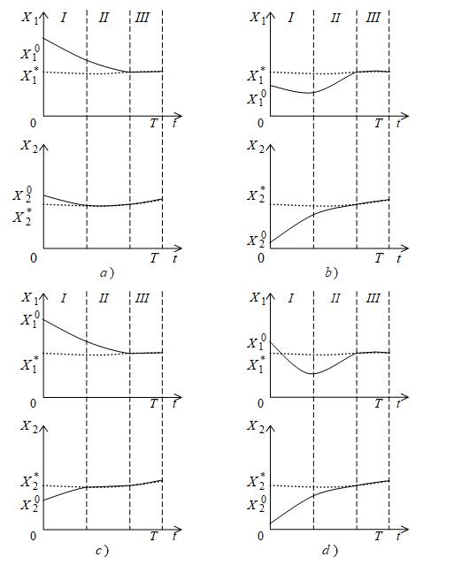
In general, the movement of the economic system along the optimal trajectory in accordance with the control strategy (9) consists of three stages.

Stage I. At this stage, the following conditions are met: $\forall i,j:\mathrm{}{q}_i{\alpha }_i\ne q_j{\alpha }_j\ne \lambda ,i,j=\stackrel{-}{\mathrm{1},n}$ (see formulas 7,8 ). Consider two cases: the set $K$ is empty or not.

Option 1. We call competing factors such factors for which $\mathrm{\Delta }>\mathrm{0}(K\ne \mathrm{0})$. If a subset $K_{\mathrm{1}}\subseteq K$ includes one index, then investments aremade only in the factor corresponding to this index. Other factors amortize $(s=\mathrm{0})$ (figure $\mathrm{1}\mathrm{b},\mathrm{d}$ ). If the subset $K_{\mathrm{1}}$ contains two or more indices, then stage $I$ is absent.

Option 2. In the absence of competing factors $(K=\theta )$ all factors amortize until at least one of the factors reaches a quasi-stationary level (figure $\mathrm{1}\mathrm{a},\mathrm{c}$ ).Stage II. Entering a quasi-stationary orbit.Option 1. At stage II, the subset $K_{\mathrm{1}}\subseteq K$ includes $m$ indices $(m\ge \mathrm{2})$. The following condition is ${\mathrm{m}\mathrm{e}\mathrm{t}}_{\text{in }}^{-}{q}_i{\alpha }_i=q_j{\alpha }_j\ne \lambda ,\forall i,j\in K_{\mathrm{1}}$. Accordingly, $\forall i,j$ competing factors the following is fulfilled: ${\mathrm{\Delta }}_i={\mathrm{\Delta }}_j>\mathrm{0}$. Investments in competing factors are made according to the rate of accumulation $\hat{s}$; investments in other factors are equal to zero (figure $\mathrm{1}\mathrm{b},\mathrm{d}$ ).

Let us construct a system for determining the control variables ${\hat{s}}_{k_{\mathrm{1}}}$ of the strategy (9). Let us introduce the notation $q_i{\alpha }_i=q_j{\alpha }_j=\chi$. Then ${\stackrel{\dot{}}{q}}_i{\alpha }_i+q_i{\stackrel{\dot{}}{\alpha }}_i={\stackrel{\dot{}}{q}}_j{\alpha }_j+q_j{\stackrel{\dot{}}{\alpha }}_j=\stackrel{\dot{}}{\chi }$.We transform the sum included in the first equation of system (5):

$\begin{array}{rr}& \underset{k=\mathrm{1}}{\overset{n}{\sum }} {\alpha }_k\left(s_k+{\beta }_k\right)q_k=\gamma \underset{k\in K_{\mathrm{1}}}{\sum } s_k+\gamma \underset{k\in K_{\mathrm{1}}}{\sum } {\beta }_k+\underset{k\in K_{\mathrm{2}}}{\sum } {\alpha }_k\beta \\ & =\gamma \left(\mathrm{1}+\underset{k\in K_{\mathrm{1}}}{\sum } {\beta }_k+\underset{k\in K_{\mathrm{2}}}{\sum } \frac{{\alpha }_k{\beta }_k{q}_k}{\gamma }\right)=\gamma \left(\mathrm{1}+\underset{k=\mathrm{1}}{\overset{n}{\sum }} \frac{{\beta }_k}{\tilde{\alpha }}\right)\end{array}$

where ${}_{{\alpha }_n}{\tilde{\alpha }}_k=\mathrm{1},\mathrm{}k\in K_{\mathrm{1}};\mathrm{}{\tilde{\alpha }}_k=\chi /\left({\alpha }_k{q}_k\right),\mathrm{}k\in N\setminus K_{\mathrm{1}}$.Then (5) will take the form:

$\left\{\begin{array}{l}\frac{\stackrel{\dot{}}{\chi }}{\chi }=\frac{{\stackrel{\dot{}}{\alpha }}_i}{{\alpha }_i}+\delta +{\gamma }_i-f_{x_i}^{\mathrm{\text{'}}}\left(\bar{x}\right){\alpha }_i\left(\mathrm{1}+\underset{k=\mathrm{1}}{\overset{n}{\sum }} \frac{{\beta }_k}{{\tilde{\alpha }}_k}\right),i\in K_{\mathrm{1}}.\\ {\stackrel{\dot{}}{x}}_i={\alpha }_i\left({\hat{s}}_i+{\beta }_i\right)f\left(\bar{x}\right)-{\gamma }_i{x}_i,\end{array}\right.$

The first equation of system (11) is valid for all competing factors. Let us subtract the first equation of the system for the factor $j$ from the same equation for the factor $i$ :

$f_{x_i}^{\mathrm{\text{'}}}\left(\bar{x}\right){\alpha }_i-f_{x_j}^{\mathrm{\text{'}}}\left(\bar{x}\right){\alpha }_j=\left(\left({\stackrel{\dot{}}{\alpha }}_i/{\alpha }_i\right)-\left({\stackrel{\dot{}}{\alpha }}_j/{\alpha }_j\right)+{\gamma }_i-{\gamma }_j//\mathrm{1}+\underset{k=\mathrm{1}}{\overset{n}{\sum }} \left({\beta }_k/{\tilde{\alpha }}_k\right)\right);i,j\in K_{\mathrm{1}}\text{. (12) }$

Expression (12) defines a hypersurface in $(n+\mathrm{1})$-dimensional space $(t,\bar{x})\in R_{+}^{n+\mathrm{1}}$.

Thus, the system for determination ${\hat{s}}_{k_{\mathrm{1}}}$ has the form:Thus, the motion at stage II is described by a system consisting of $\mathrm{2}m$ equations: $(m-\mathrm{1})$ hypersurface equation ${\mathrm{\Phi }}_i(t,\bar{x})=\mathrm{0},\left(m\right)$ phase equations $\stackrel{\dot{}}{\bar{x}}=\phi (t,\bar{x})$ and the constraint equation for the control variables ${\sum }_{k_{\mathrm{1}}} {\hat{s}}_{k_{\mathrm{1}}}=\mathrm{1}-{\sum }_{k=\mathrm{0}}^n {\beta }_k:\left\{{\mathrm{\Phi }}_i(t,\bar{x})=\mathrm{0},\stackrel{\dot{}}{\bar{x}}=\phi (t,\bar{x}),{\sum }_{k\stackrel{-}{\mathrm{1}}} {\hat{s}}_{k_{\mathrm{1}}}=\mathrm{1}-{\sum }_{k=\mathrm{0}}^n {\beta }_k\right.$.

Thus, the motion at stage II is described by a system consisting of $\mathrm{2}m$ equations: $(m-\mathrm{1})$ hypersurface equation ${\mathrm{\Phi }}_i(t,\bar{x})=\mathrm{0},\left(m\right)$ phase equations $\stackrel{\dot{}}{\bar{x}}=\phi (t,\bar{x})$ and the constraint equation for the control variables ${\sum }_{k_{\mathrm{1}}} {\hat{s}}_{k_{\mathrm{1}}}=\mathrm{1}-{\sum }_{k=\mathrm{0}}^n {\beta }_k:\left\{{\mathrm{\Phi }}_i(t,\bar{x})=\mathrm{0},\stackrel{\dot{}}{\bar{x}}=\phi (t,\bar{x}),{\sum }_{k_{\mathrm{1}}} {\hat{s}}_{k_{\mathrm{1}}}=\mathrm{1}-{\sum }_{k=\mathrm{0}}^n {\beta }_k\right.$.

Option 2. The following condition is met $\forall i,j:q_i{\alpha }_i<q_j{\alpha }_j=\lambda (N=I\cup J)$. Control variables with indices $i\in I:q_i{\alpha }_i<\lambda$ take values $s_i=\mathrm{0}$, the relevant factors amortize as long as the coefficients $\mathrm{\Delta }\ne \mathrm{0}$. The control parameters with indices $j\in J:q_j{\alpha }_j=\lambda$ take values $s_j=s_j$ (figure $\mathrm{1}\mathrm{a},\mathrm{c}$ ). When the condition $\mathrm{\Delta }=\mathrm{0}$ is fulfilled for all factors, the transition to the third stage is carried out.

Stage III. Motion along a quasi-stationary trajectory. At this stage, all $\mathrm{\Delta }=\mathrm{0}(N=J)$, dual estimates satisfy condition (15), i.e $\forall i,j:q_i{\alpha }_i=q_j{\alpha }_j=\lambda ,i,j=\stackrel{-}{\mathrm{1},n}$. Stage III involves the fulfillment of equality $s_j=s_j^{\mathrm{*}}$ (Figure 1).

See Full Size >

Conclusion

The problem of constructing the process of managing the economic system with the possibility of taking into account an arbitrary finite number of factors influencing its development is solved. The criterion for improving the well-being of the population and the quality of life against the background of sustainable economic growth was adopted as an optimization criterion.

In the formulation of the problem, indicators are introduced that take into account the level of specific efficiency of investments in the factors of development of the economic system. An algorithm is proposed for the optimal distribution of investments that maximizes the optimization criterion over a given time interval. The solution to the optimal planning problem is found using a combination of analytical and numerical methods. The algorithm for constructing the optimal control includes three stages. All variants of trajectories possible combinations for factors dynamics are considered, proceeding from their values at the initial moment of time.

Thus, the mathematical apparatus for describing multidimensional models of macroeconomic dynamics is presented. The parameters of the quasi-stationary trajectory are determined, the strategy of optimal control of production factors is built. The resulting algorithm can be used in real calculations to build strategies for optimal control of economic systems with an arbitrary number of factors.

References

• Agarkov, G. A., & Tarasyeva, T. V. (2020, November). Estimation of economic system’s proportional development using economic growth model. In AIP Conference Proceedings (Vol. 2293, No. 1, p. 120003). AIP Publishing LLC.

• Alonso-Carrera, J., Bouché, S., & de Miguel, C. (2021). Revisiting the process of aggregate growth recovery after a capital destruction. Journal of Macroeconomics, 68, 103293.

• Belenkii, V. Z. (2016). Optimal Management: the Maximum Principle and Dynamic Programming, 132.

• Belenkii, V. Z., & Ketova, K. V. (2006). Full analytical solution of a region development macro model under an exogenous demographic prognosis, Economics and matematical methods, 42(4), 85-95.

• Cass, D. (1965). Optimum Growth in an Aggregative Model of Capital Accumulation. Review of Economic Studies, 32, 233-240.

• Davydenko, N., Dibrova, A., Onishko, S., & Fedoryshyna, L. (2021). The influence of the gross regional product on the formation of the financial potential of the region. Journal of Optimization in Industrial Engineering, 14(1), 177-181.

• Esfandiari, M. (2020). Dynamic optimization of capital stock: An application of maximum principle. Industrial Engineering and Management Systems, 19(3), 589-596.

• Grigorenko, N., & Luk’yanova, L. (2021). Optimal control and positional controllability in a one-sector economy. Games, 12(1), 1-12.

• Ioffe, A. D. (2020). An Elementary Proof of the Pontryagin Maximum Principle. Vietnam Journal of Mathematics, 48(3), 527-536.

• Ketova, K. V., Rusyak, I. G., & Derendyaeva, E. A. (2013). Solution of the Problem of Optimum Control Regional Economic System in the Conditions of The Scientific and Technical and Social and Educational Progress. Mathematical modeling, 25(10), 65-78.

• Ketova, K. V., & Saburova, E. A. (2020). Addressing a problem of regional socio-economic system control with growth in the social and engineering fields using an index method for building a transitional period. Advances in Intelligent Systems and Computing. Software Engineering Perspectives in Intelligent Systems, 385-396.

• Kiselev, Y. N., Avvakumov, S. N., Orlov, M. V., & Orlov, S. M. (2020). Optimal Resource Allocation in a Two-Sector Economy with an Integral Functional: Theoretical Analysis and Numerical Experiments. Computational Mathematics and Modeling, 31(2), 190-227.

• Koopmans, T. C. (1965). On the Concept of Optimal Economic Growth. Pontificae Academiae Scientiarum. Scripta Varia, 28, 225-300.

• Polat, G. G., & Ozer, T. (2020). On group analysis of optimal control problems in economic growth models. Discrete and Continuous Dynamical Systems - Series S, 13(10), 2853-2576.

• Pontryagin, L. S., Boltyansky, R. V., Gamkrelidze, V. G., & Mishchenko, E. F. (1961). Mathematical theory of optimal processes, 391.

• Ramsey, F. P. (1928). A Mathematical Theory of Saving. Economic Journal, 38(152), 543-559.

• Ren, M., Chen, J., Shi, P., Yan, G., & Cheng, L. (2021). Statistical information based two-layer model predictive control with dynamic economy and control performance for non-Gaussian stochastic process. Journal of the Franklin Institute, 358(4), 2279-2300.