
Modern Geoinformation And Communication Technologies Of Economic Analysis In Ms Office 365


Abstract
The article considers new geographic information and communication capabilities of MS Office 365 when used in economic analysis. The aim of the research is the development of digital mapping technology in the presentation of data of economic analysis and determination of the composition of rents, defining the productivity of geographically distributed production using a specific real statistical data. Technologies for the presentation of economic data in the form of digital Bing, 3D, and custom maps have been developed, as well as technologies of adding digital Bing maps, visualization of data illustrating the effect of rental factors on milk production in some regions of the Russian Federation. These factors are determining differential rent I (DRI), determining differential rent II (DRII), factors of administrative status (corruption) rent (ASR), factors of absolute (speculative) rent (AR). Among the standard sets of thematic mapping types, visualization in the form of a heat map is considered as the most suitable one. However, it is not recommended for practical usage due to low accuracy, instead, it is suggested to use the standard Excel-Surface diagram. On the basis of the developed technologies, rental analysis of production productivity was carried out: the authors got an equation of regression depending on the productivity of milk production on the rental proportions of DRII, DRI, ACP, AR; the values of rents corresponding to each of the rental proportions, and total rent were found. The article proves the leading position of the proportions of differential rent II (DRII) to determine the production efficiency.
Keywords: Differential rent IIdigital mappingeconomicsinformation and communication capabilitiesmanufacturingMS Office 365
Introduction
To the present moment, the enhanced capabilities of MS Office 365 have been implemented by the following main tools, which allow performing economic analysis at the space-time level (Rudikova, 2017):
Mapping with the use of standard geographic web maps.
Working in a local network, intranet and Internet.
Developing web-sites, work in HTML / MHTML format.
Working with data in XML format, answering web requests.
Recently, the rent-based theory of production regulation has been intensively developed both at the sectoral and territorial levels (Zaitsev, 2017, 2016, 2015; Efimova, Yarmolenko, & Isaev, 2014; Efimova, Yarmolenko, & Efimova, 2011; Yarullin, 2002). The concept of rent as part of the productivity of production is expanding. At the same time, each rent affects the productivity in proportion, and this influence is determined by the proportion of the corresponding rent – the rental ratio. In our opinion, complementary to modern studies (Zaitsev, 2017, 2016) is a study of the ranking of rents and their impact on productivity, which would allow identifying specific political and economic factors of production increase corresponding to these rents.
Problem Statement
In the conditions of the development of digitalization of the economy and the expansion of the use of modern software products for analysis and reasonable management solutions to improve production efficiency, it seems necessary, to develop tools for using modern digital mapping capabilities for presenting economic data and conducting rental analysis.
Research Questions
The following research questions are posed:
Development of technologies for the presentation of economic data based on geo-information in the form of digital Bing-maps, 3D-maps, custom maps.
Rental analysis of production efficiency using geo-information data in order to identify rental proportions that determine the level of production.
Purpose of the Study
The purpose of this article is the development of digital mapping technology in the presentation of economic analysis data and determination of the composition of rents that define the production efficiency on a specific real statistical material.
Research Methods
The research was carried out with the methods of analysis and synthesis, economic-mathematical and geo-information modeling.
Findings
At present, digital geographic maps are widely used for economic and social analysis in order to make effective management decisions. In this regard, digital maps of Microsoft Office Excel 2016 are of practical importance. In this system, they are defined as add-ins:
Bing digital maps;
3D Maps;
custom maps.
In order to determine the possibility of using Microsoft Office Excel 2016 for geoinformation analysis, we will consider each of the settings for practical application for geoinformation analysis (GIA) of socio-economic phenomena.
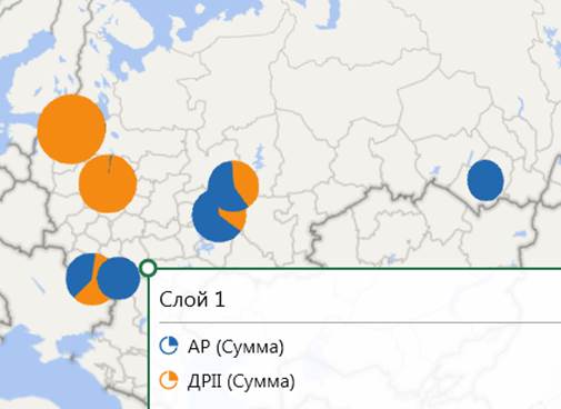
Working with the Bing Digital Map Add-in
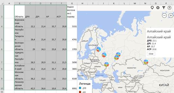
We use this option to visualize data illustrating the effect of rental factors on milk production in some regions of the Russian Federation (Zaitsev, 2017). These factors include (Table
factors that determine the differential rent (DRI);
factors determining the rent (DRII);
factors of administrative status (corruption) rent (ASR);
factors of absolute (speculative) rent (AR).
In this first map variant, the following commands are executed in sequence:
Insert → My add-ons → Watch (Вставка → Мои надстройки → Смотреть),
Office add-ons (Надстройки Office) → select Bing Maps (Карты Bing),
select the data in the Excel spreadsheet and execute the command Show locations (Показать местоположения).
As a result, we get a thematic map of the influence of rental factors by region (Figure
Work with 3D Map add-in
The second map construction variant (3D map) is done by the sequence:
Insert → 3D Map → Open 3D-Maps (Вставка → 3D-Карта → Открыть 3D-Maps (Карты));
by selecting the data in the Excel table, execute the Add selected data to 3D Maps (Добавить выбранные данные в 3D Maps) command;
in the window Overview “No.” (Обзор «№») on the “Fields List” («Список полей») tab, execute the command Drag the fields to the layers panel (Перетащите поля на панель слоев;); with this command the field the Data Area (Область) is transferred to the Location (Расположение) field of the layer panel, since each country, district, region / kray (federation subject), city, street corresponds to a position on the map defined by geographic latitude and longitude;
in the Height (Высота) field of the layers panel by clicking on the plus-shaped label all fields of thematic data are entered alternately;
the “Layer Parameters” («Параметры слоя») mode sets the graphic parameters, and by turning on the regional map visualization (визуализации региональной карты) mode, the boundaries of the corresponding administrative unit are displayed with all thematic data (Figure
02 ).
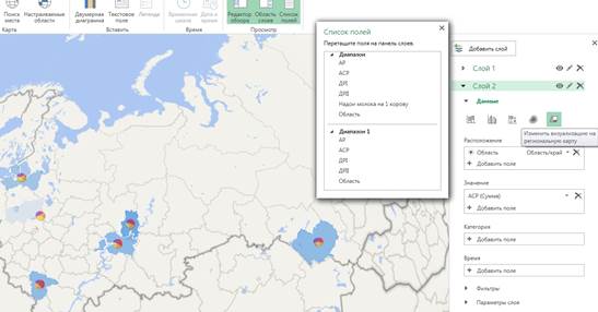
The color density of the administrative unit characterizes the value of the current parameter - in this case, the value of the ASR.
Making custom maps
Custom maps can solve a wider range of tasks than digital Bing cards and 3D maps. They easily adapt to any particular tasks and occupy less space in the computer’s memory. In addition, the researcher can define his/her own rectangular coordinate system, which cannot be done in the above-mentioned digital maps. Custom maps are created for point and area objects, and area objects (user areas) should be created in the format shp (Shapefile), i.e. as shapefiles used in the ArcGis system (by ESRI USA), as well as in kml (Keyhole Markup Language File) format for representing three-dimensional geospatial data in Google Earth. Let us show the order of creating a custom map using the example of point objects.
1. Custom maps are created on a raster substrate base made in any standard raster format. In our example, such a substrate is created in the form of a file
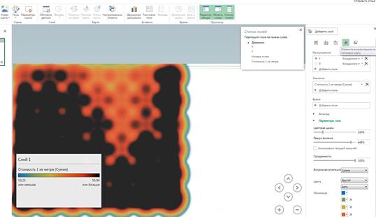
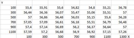
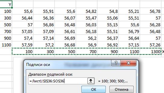
2. Given the screen coordinate system (the y axis is directed downward with the normal x axis direction), we construct a thematic map of the cost of one square meter of land - the specific indicator of land cost (SILC) - on the points of the regular grid shown in the Excel table (Figure
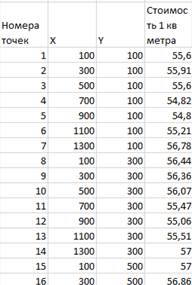
In Figure
3. The technology of making a custom map comes down to the following successive operations:
Insert → 3D Map → Open 3D-Maps → New scene → Create a custom map (Вставка → 3D-Карта → Открыть 3D-Maps(Карты) → Новая сцена → Создать пользовательскую карту);
in the Custom Map Settings (Параметры пользовательской карты) window execute the command Import Picture as a background map for your data (Импортировать рисунок в качестве фоновой карты для ваших данных); for this purpose, the previously prepared substrate file IsobPolzKarty.jpg (ИзобПользКарты.jpg) is imported;
by executing the command Space of pixels (Пространство пикселей), the system of rectangular coordinates of the screen is set; the commands Turn the axis; Swap the X and Y axes (Перевернуть ось, Поменять местами оси X и Y); the coordinate system can be changed as desired; after the execution of the Apply, Finish (Применить, Готово) commands, the coordinate system will be set finally;
by running the standard command Insert → 3D-Map → Open 3D-Maps → (Вставка → 3D-Карта → Открыть 3D-Maps(Карты) →) (after highlighting the data in the Excel table) Add the selected data to 3D Maps (Добавить выбранные данные в 3D Maps);
on the “List of fields” («Список полей») tab, execute the command Drag fields to the layers panel; at the same time, put the X field in the Location section in accordance with the Coordinate on the X axis, and the Y field in the Y axis coordinate, the Point number fields and the Cost per 1 square meter move to the Height section;
on the “List of fields” («Список полей») tab, execute the command Drag fields to the layers panel (Перетащите поля на панель слоев); at the same time, put the X field in the Location section in accordance with the Coordinate on the X axis (Координата по оси X), and the Y field – on the Y axis coordinate (Координата по оси Y), the Point number (Номера точек) fields and the Cost per 1 square meter (Стоимость 1 кв метра) move to the Height (Высота) section;
in the section of diagrams, it is necessary to execute the Change visualization to heat map (Изменить визуализацию на тепловую карту) command; in the Parameters section of the layer, set the Value of the color scale (Значение цветовой шкалы) to 103%, and the Radius of influence to 448%; it is also recommended with the Add Color (Добавить цвет) command select the six colors of the present diagram with the color transition from the minimum value of the SILC to the maximum.
The resulting diagram (Figure
Further on, the algorithm for constructing the surface will be as follows.
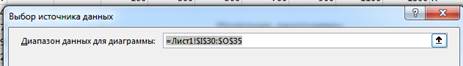
1. After data capture, execute the command Insert → Maps → Other charts with maps (Вставка →Карты → Другие диаграммы с картами) (Figure
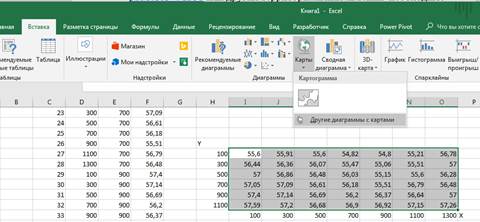
2. Select the
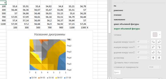
To sign the coordinates, right-click on the diagram and get a pop-up menu in which choose the
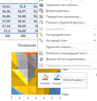
With the
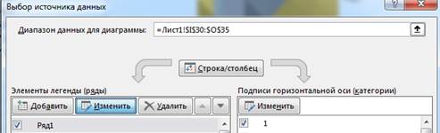
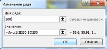
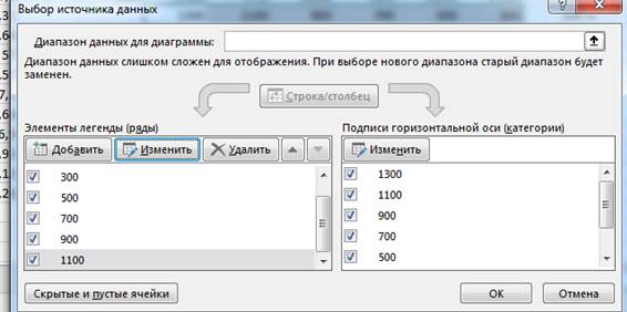
To replace X values, execute the
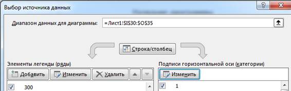
After entering OK, we will receive a new view of the
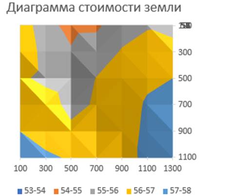
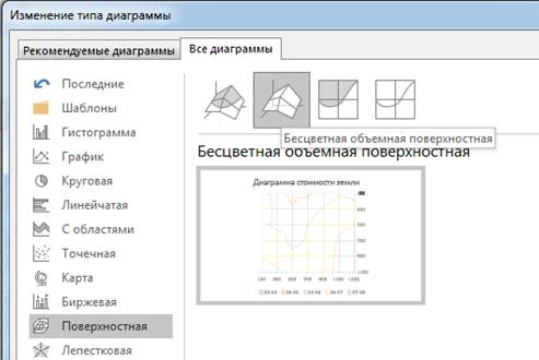
The surface diagram has the following positive properties:
It is accurate. The chart model does not introduce modeling errors in contrast to the thermal model. Its accuracy depends only on the accuracy of the source data.
All zones are clearly distinguished by colors and isolines in contrast to the blurred zones of the heat map; the colors of the zones can be changed by standard means.
It is possible to build a map of isolines, change their thickness, color and other parameters.
Rental analysis of production efficiency
For the implementation of rental analysis of livestock productivity, shown in Figure
Such an equation will be the basis for calculating the above rents: DRII, DRI, ASR, AR. According to Figure
У= 182.9 * DRII + 25.9 * DRI + 56.2* ASR – 114.2 * AR,(1)
with the coefficient of determination of the model equal to 0.98 and the calculated value of the F-criterion equal to 41.6 with the threshold value of this criterion with 3 degrees of freedom and significance level of 0.05 equal to 8.9.
The value of the rent corresponding to the rental factor i, we find the following way:
Рi = Уact.i; min.j,k,l – Уmin. I,j,k,l,(2)
where Уact.i; min.j,k,l – efficiency at the actual value of factor i and the minimum values of factors j, k, l;
Уmin. I,j,k,l – efficiency at the minimum values of all factors.
As an example, let us show the calculation of the rent corresponding to a certain rental factor or rental ratio.
In Table
Performing similar calculations for each rental ratio, we will create a general table of calculated rents and find the total rent as a row-wise sum of values (Table
On the basis of Table
Conclusion
This article solves the problem of developing technology for digital mapping of regional economic data in MS Office 365, and also proves the leading position in the productivity of production of geographically distributed proportions on the digital map defining DRII. The developed technologies can be used in educational modules, in the parts of the educational process related to the analysis of geographically distributed economic and social data.
References
- Efimova, G. A., Yarmolenko, A. S., & Isaev, G. A. (2014). Rental analysis of the causes of the agrarian crisis in Russia. Land Management, Cadastre and Land Monitoring, 7, 15-21.
- Efimova, G. A., Yarmolenko, A. S., & Efimova, S. V. (2011). Rental foundations of land management in the regional economy (theoretical aspect). Veliky Novgorod: Yaroslav-the-Wise Novgorod State University.
- Rudikova, L. V. (2017). Microsoft Office Excel 2016. St. Petersburg: BHV-Petersburg.
- Yarullin, R. R. (2002). The mechanism of redistribution of land rent in a market economy. International Agricultural Journal, 2, 7-10.
- Zaitsev, A. A. (2017). Rent regulation of agrarian relations sustainability: regulatory dynamic approach. (Doctoral dissertation). Moscow: Economics and Management of National Economy.
- Zaitsev, A. A. (2016). Rental problems of import substitution in the agricultural sector of the Russian economy. Economics of Agricultural and Processing Enterprises, 5, 25-29.
- Zaitsev, A. A. (2015). Rental problems of the effectiveness of state support in the agricultural sector of the Russian economy. News of the International Academy of Agrarian Education, 2(25), 54-60.
Copyright information

This work is licensed under a Creative Commons Attribution-NonCommercial-NoDerivatives 4.0 International License.
About this article
Publication Date
02 April 2019
Article Doi
eBook ISBN
978-1-80296-058-7
Publisher
Future Academy
Volume
59
Print ISBN (optional)
-
Edition Number
1st Edition
Pages
1-1083
Subjects
Business, innovation, science, technology, society, organizational theory,organizational behaviour
Cite this article as:
Yarmolenko, A., Putintseva, N., & Pisetskaya, O. (2019). Modern Geoinformation And Communication Technologies Of Economic Analysis In Ms Office 365. In V. A. Trifonov (Ed.), Contemporary Issues of Economic Development of Russia: Challenges and Opportunities, vol 59. European Proceedings of Social and Behavioural Sciences (pp. 643-656). Future Academy. https://doi.org/10.15405/epsbs.2019.04.69