Spatial Stochastic Frontier Analysis Of Russian Regions Development From 2011 To 2016

Abstract

Most of the previous studies estimated technical efficiency for special industries, not considering Russian territory as a whole. This article provides technical efficiency estimates for 78 Russian regions. Alongside with traditional factors such as labour and capital, the authors took into account a nontrivial factor seen as retail trade. Retail trade had been chosen since it ultimately creates a technology demand. We also added spatial effects into a stochastic frontier model considering spatially related efficiency. The authors estimated stochastic frontier models with three-factor production function and spatially related efficiency for Russian regions, viewing the last six years from 2011 to 2016. Thus helped to analyse regions’ technical efficiency evolution before the influence of implied sanctions (2014) and after it. The outcome proved that technical efficiency decreases in the analysed period. The technological development of Russian regions is characterized by high variability and territorial heterogeneity. The level of regions’ technical efficiency varies so much that we can talk about geographically distributed zones. Regions with the highest level of technical efficiency are concentrated in Western Siberia, the Urals, the European part along the Volga River and Southern Federal districts. Regions with low technical efficiency are located within Western and Eastern borders of Russia. The leading regions development is slowly reorganizing due to innovations. The role of invention and high-performance production expansion gradually increases. This trend has not been observed yet for weak regions.

Keywords: Technical efficiencyspatial stochastic frontier analysisinnovationseconomic sanctions

Introduction

Russian Federation consists of 85 regions (also referred as federal subjects of Russia). All the regions differ in many aspects especially because of different areas, geographical positions and climatic zones.

At present the quantity of Russian economy studies assuming regional interaction is drastically low although considering spatial effects is simply natural.

In addition, besides including the spatial effects we should also consider consistence of Russian economy development. Geographical distribution of industrial activity in Russia was strictly specified by the former type of centrally planned economy. But since 1991 the roles of regions and their development level changed a lot. Decline and stagnation of 1990th resulted in 1998 with deep economic crisis. Further situation gradually improved. Until 2008 most regions have demonstrated fast growth. But by then many problems had arisen, including low technological development, imbalance in income distribution between the regions, domination of extraction and retail branches over industry and manufacturing.

Nowadays Russian economy weakly demonstrates recovery growth. Russia urgently has to search for sources of sustainable economic development. This transition should be based upon the more profound use of regional resources.

Since 2014 the regional development problem has intensified due to influence of external restrictions (sanctions). Sanctions disrupt the ability to update material and technical base and create demand for innovation. One of the driving forces of regional economies, especially in developing countries (Henry, Kneller, & Milner, 2009) including Russia, is technological development, now restrained by sanctions.

Under these conditions the technical efficiency evolution study of the Russian regions becomes particularly relevant both in the pre-sanction period and in the initial active phase of external restrictions. We attempt to characterize the response of each region to these sanctions by estimating its technical efficiency.

Problem Statement

The study of estimating the regions’ technical efficiency is observing the following features.

First, unlike most studies, the authors decided to focus on the regions as territorial integrities and socio-economic systems. The problem of the technical efficiency estimates of farms (Saraikin & Yanbykh, 2014), economy sectors, countries (Mamonov & Pestova, 2015) has been repeatedly studied. Various specifications of technical efficiency models were used depending on various factors reflecting upon the study of economic efficiency (labour, human capital, institutional factors, resource rent, etc.).

Secondly, we will make an attempt to analyse the Russian regions technical efficiency by means of adaptation to external economic sanctions considering the role of spatial effects. Along with such traditional factors as labour and intellectual capital (Makarov, Ayvazyan, Afanasyev, Bakhtizin, & Nanavyan, 2014) the factor of retail trade was introduced. This factor indirectly characterizes the innovative products demand and thus contributes to technological activity.

The competitive advantages theory contributed to the revealing influence of spatial proximity, territorial clusters and agglomerations in technological development. In this context, the role of non-material factors related to the business climate is crucial. They stimulate the knowledge accumulation and flow between the nearby territories. In some cases, the availability of these mechanisms ensures new production methods and technologies diffusion. This brings us closer to the technological frontier. The ideas of the P. Krugman’s new economic geography developed the applied direction of spatial econometrics. It marked the beginning of a new cycle of scientific works (Krugman, 2010). These works proved acknowledgement of the spatial factor, i.e. neighbourhood, distance and macroeconomic indicators of other territories (Di Guardo, Marrocu, & Paci, 2016). However, geographical proximity itself is neither a necessary nor a sufficient condition for increasing innovation activity in the region. It can facilitate the interactive exchange of knowledge and technology or, conversely, have a negative impact on innovation (Boschma, 2005).

Third, unlike similar studies (Fusco & Vidoli, 2013), we estimated technical efficiency over the 2011-2016 years, not by using the panel data. Thus, we wanted to show the technical efficiency evolution for Russian regions before and after 2014. The period of 2011-2016 allowed to cover the recovery stage of the Russian economy after the crisis of 2008-2009, as well as to recognize the continuing opposing influence of economic sanctions and retaliatory measures imposed against Russia in 2014.

Research Questions

From a practical point of view, the study aims to address the following issues:

• what are the levels and changes of technical efficiency in the analysed period;

• is it possible to distinguish the spatial zones of regions with a similar level of technical efficiency;

• what is the dynamics of the innovative factors influence such as the number of high-performance jobs, inventive activity etc.

• The answers to these questions allow us to develop more accurate measures of regional innovation and foreign economic policy.

Purpose of the Study

We will show the technical efficiency evolution for Russian regions through 2011-2016 thus identifying sustainable spatial patterns, characterized by homogeneity of technical efficiency. Then we will search for factors that affect technical efficiency of regions. We propose it can be formed by some innovative factors (like inventive activity, the number of high-performance jobs) and spatial factors (such as the knowledge and technology flow).

Research Methods

Model description

In this paper, the technical efficiency is defined as the ability to obtain the maximum potential output from a given input vector. Formally, technical efficiency is measured as the ratio of the observed output to the potential output (frontier output).

There are two major approaches for estimating technical efficiency. The first one is deterministic Data Envelopment Analysis (DEA), the second one is Stochastic Frontier Analysis (SFA). It should be noted that their direct comparison is difficult, since DEA is deterministic and avoids SFA specification errors and problems associated with model parameter estimates due to factors multicollinearity. The method choice largely depends on the specific purpose. For example, some researchers noted the advantage of using DEA for the analysis of certain industries. Others admitted that the levels of technical efficiency estimated by DEA and SFA differ. In some cases, DEA gives higher technical efficiency estimates, sometimes the situation is opposite (Hjalmarsson, Kumbhakar, & Heshmati, 1996; Odeck & Brathen, 2012; Malakhov & Pilnik, 2013). In this paper author chose spatial SFA within the study purpose.

There are usually four types of spatial effects adding to a linear stochastic frontier model used to compare the regions performance (Pavlyuk, 2014): endogenous and exogenous spatial effects, spatially correlated errors and spatially related efficiency. Endogenous and exogenous spatial effects are well-known and widely used (Ramajo & Hewings, 2018; Glass, Kenjegalieva, & Sickles, 2016). The fourth type of spatially related efficiency is rather new (Areal, Balcombe, & Tiffin, 2012; Fusco & Vidoli, 2013).

In the current research, we need to eliminate the neighbouring regions inefficiency interaction of the technical efficiency estimates. So, the model with spatial effects of the fourth type was accepted as follows:

See Full Size >

Gross regional product per capita for 78 Russian regions from 2011 to 2016 ( GRP ) is taken as an endogenous variable; the assumed factors were seen as:

• fixed assets at the residual value per employed person in the economy ( K ),

• the average employed persons share in the total population of the year ( L ),

• retail trade turnover per employed person in the economy ( T ).

See Full Size >

is square symmetric weight matrix characterizing the spatially related efficiency; n is the number of regions; and

See Full Size >

is the parameter characterizing the spatial correlation.

We took 78 of 85 Russian federal subjects for the following reasons. First, we eliminated the Chechen Republic and the Republic of Ingushetia because we cannot trust the statistics of those regions. Secondly, Yamalo-Nenets Autonomous Okrug and Khanty-Mansiysk Autonomous Okrug – Yugra were considered jointly with Tyumen oblast. Similarly, Nenets Autonomous Okrug statistics was included in the Arkhangelsk Oblast data. Third, we eliminated The Republic of Crimea and Sevastopol.

The spatial effects weight matrices construction is usually considered an empirical problem. However, many studies have shown that these matrices significantly affect the estimation results (Areal et al., 2012). Within the purpose of the study and since the model includes spatial effects, it is estimated not on panel data, but for each year separately. The models are calculated with three types of weight matrices.

The first type is the simplest nearest neighbor weights method where

See Full Size >

if the regions are neighbours, and 0, in other case. The second one is power distance weights method. We take geographical coordinates for subjects’ capitals. Then we calculate the distances

See Full Size >

between them, and finally

See Full Size >

,

See Full Size >

or

See Full Size >

This type also include a variation when

See Full Size >

are calculated as the distances between the capitals by road (Balash, 2012). The third type of weight matrices is exponential distance weights method.

See Full Size >

are calculated as in the previous one, but

See Full Size >

. The matrix is normalized so that the sum of each row is equal to one. The calculations showed that the first nearest neighbour weights method gives the most stable results. So, the 6th section of the paper presents the calculations results obtained using this type of spatial matrix.

Models with larger number of factors were also considered. We tried to include the investment in fixed capital (with the lag of one and two years), the industrial production index, as well as the employed population share aged 25-64 with higher education in the total employed population of the corresponding age group. The results were unsatisfactory due to the high factors collinearity, so these factors were eliminated from the model. The parameter estimates were insignificant, and the spatial effect parameter estimation was unstable (the condition of

See Full Size >

was violated).

The technical efficiency calculation was carried out according to the Battese and Coelli formula (Battese & Coelli, 1988). The maximum likelihood estimation was executed using the Spfrontier package of R .

Findings

Russian regions technical efficiency evolution

Table 01 shows modelling results for 2011-2016. All parameters are significant at the level of at least 0.001. Figure 02 shows how parameter estimates change from 2006 to 2011.SSFA model estimation results.

See Full Size >

See Full Size >

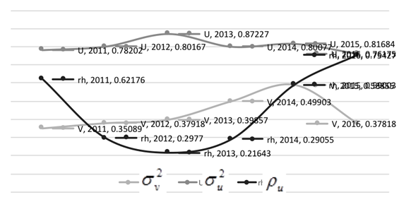
Note that the

See Full Size >

parameter value responsible for the spatial correlation between the regional efficiencies decreases to 0.2 in 2013 and recovers above the level of 2012 (0.75) in 2016. Ultimately, the impact of random factors representing inefficiency from neighbouring regions increased. So, it reduced the production potential of the regions. It should be also noted that a similar pattern of spatial correlation was observed in most models with another factors. In turn, the Moran’s I confirms positive spatial correlation for the technical efficiencies themselves and it is significant for all six years (see Table 02 ).

See Full Size >

In contrast to the prosperous period of 2011-2013, the period of 2014-2016 represents the development of the processes determining the values clustering in neighbouring regions (there is an increase of Moran's I ). More developed regions tend to the similar ones and vice versa. This may indicate a necessity increase for interregional cooperation in difficult economy periods.

The Moran scatterplot allows to distinguish four quadrants of regions by the level of technical efficiency. In the first quadrant, we can find high-efficiency regions surrounded by high-efficiency neighbours (HH). In the third quadrant, there are low-efficiency regions which are surrounded by low-efficiency neighbours (LL). In second (LH) quadrant we can find the group of low-efficiency regions with high-efficiency neighbours and in fourth (HL) quadrant there is the opposite situation. In general, in 2011-2016 there is a decrease in the level of technical efficiency. Table 03 represents the median values of technical efficiency for each Moran’s quadrant by year, the second-line value in each cell is the number or regions in each quadrant by year.

See Full Size >

For each quadrant, the median value of technical efficiency declined sharply in 2015 and continued to decline in 2016. Moran scatterplots for 2011-2016 and other detailed results of this study can be obtained in authors’ preprint (Semenychev, Khmeleva, & Kozhukhova, 2018).

We compared obtained values of technical efficiency by years (see Fig. 02 ). We also calculated sample characteristics on the averaged values of regions technical efficiency for 2011-2013 and 2014-2016 periods (see Table 04 ).

See Full Size >

See Full Size >

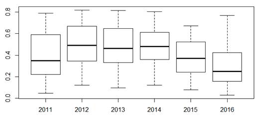
The efficiency minimum (approximately 0.1) almost hasn’t changed after the sanctions since 2014, and the maximum is reduced from 0.8 to 0.7. The values of the sample median, the first and third quartiles have significantly decreased. The efficiency distribution is asymmetrical, and the skewness value increases. Regardless of the sanctions, the technical efficiency distribution is bimodal, which does not contradict the known results (Mamonov & Pestova, 2015).

The year-by-year calculation allowed us to identify stable clusters of regions that show high technical efficiency values. This group of regions includes: Moscow, Altai Krai, Perm Krai, Krasnoyarsk Krai, the Republic of Tatarstan, The Republic of Bashkortostan, Udmurtia, The Chuvash Republic, The Republic of Mordovia, Chelyabinsk Oblast, Kemerovo Oblast, Moscow Oblast, Novosibirsk Oblast, Omsk Oblast, Orenburg Oblast, Rostov Oblast, Samara Oblast, Saratov Oblast, Tomsk Oblast, Tyumen Oblast, Ulyanovsk Oblast, Vladimir Oblast and Volgograd Oblast. Sverdlovsk Oblast improved its position and moved from the second to the first quadrant of high-efficiency regions.

By 2016 we’ve had clearly defined geographical zones of regional clusters. A large cluster of regions with high technical efficiency values surrounded by neighbours with a similar technical efficiency level (HH Moran’s quadrant) covers the border regions of Western Siberia, the Urals, the European part of the Volga River and Southern Federal districts. These regions are affected by a favourable combination of the resource base (capital, labour, natural resources) and the retail trade level. This fact helped to maintain their technical efficiency at a high level. In most of these regions there are large agglomerations, the largest mining and processing enterprises. Some regions of this cluster have external borders and developed transport corridors with Kazakhstan.

Clusters of the second and fourth Moran’s quadrants are clearly adjacent to the cluster of the first quadrant. These regions are forming a transition zone from high to low values of technical efficiency. These are mainly internal regions, and regions that border with countries with low mutual trade. Finally, by 2016, the technical efficiency evolution contributed to the formation of third quadrant regions clusters.

After 2014 a lot of regions proved to be in the third quadrant. In 2016, there are two characteristic sets of border regions and their neighbours located polar along the Western and far Eastern borders of the country. Particular attention should be paid to the regions that have moved to a group with a higher value of technical efficiency. Only Sverdlovsk region has improved its position. It can be assumed that this is a region where the policy of industrial and innovative development is successfully implemented.

In 2016 there is a group of regions of LL quadrant with low values of technical efficiency: Ivanovo Oblast, Kostroma Oblast, Ryazan Oblast, Tula Oblast and Yaroslavl Oblast.

Estimating factors impact on the Russian regions technical efficiency

We have compiled correlation matrices for 2011-2016 and identified the most significant factors influencing technical efficiency. Using the official Rosstat data from the section “Efficiency of the Russian economy”, we systematized the factors influencing the regions technical efficiency: infrastructure, industrial, innovative factors, as well as the actual efficiency of the regional economy. Considered factors are listed in the subsection 5.2 of the article. We found that there is a multicollinearity between factors high_perf_jobs , patent , research_exp . We checked the significance of the correlation coefficients between technical efficiency and chosen factors by calculating the t -statistics in the Table 05 .

See Full Size >

Thus, for all three years, the following innovative factors were significant: the number of high-performance jobs, the share of domestic expenditure on research and development in GRP, as well as the number of domestic patent applications for inventions filed in Russia.

Let’s define the significant influence factors within clusters. The clusters of HH and LL quadrant regions are the most numerous and interesting from the analytical point of view. We’ll show the influence of only those factors that were significant simultaneously in both clusters. They are the number of domestic patent applications and the number of high-performance jobs.

Figures 03 and 04 show the correlation coefficients dynamics for factors calculated within regions in quadrants HH and LL. It can be seen that the higher is the technical efficiency of the region, the greater is the impact of inventive activity and the number of high-performance jobs.

See Full Size >

See Full Size >

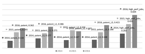
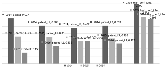
The downward dynamics of innovation factors in LL quadrant of regions can be attributed to the low efficiency of regional innovation policy in the newly included regions and the low innovation potential of its permanent participants. Regions of the HH quadrant increase inventive activity and successfully solve the problem of creating high-performance jobs.

Conclusion

By calculating technical efficiency estimates for each year, we can determine how its dynamics changes through 2011-2016. Years before sanctions (2011-2013) show its growth in all groups of regions. On the contrary, in 2014-2016 technical efficiency estimates decrease.

We also identified the time-stable spatial groups of regions with similar levels of technical efficiency.

In 2014-2016 the influence of spatial effects grows. Such tendency may reflect strengthening of inter-regional knowledge and technologies exchange in the context of restricted relations with the outside world.

Regions with high values of technical efficiency surrounded by the same-level neighbours are concentrated in Western Siberia, the Urals, the European part of the Volga River and Southern Federal districts. These regions have significant industrial, scientific and technical potential, high management experience, strong university system, the optimal distance for diffusion of innovation. As for regions with low values of technical efficiency surrounded by the same-level neighbours, there are negative institutional conditions and remoteness from innovation centres.

Further to the Western and Eastern borders of Russia there is a transition to the zone of weak regions with strong neighbours and then to weak regions with weak neighbours (LH and LL quadrants respectively). In our view, there are two reasons for this fact.

First, Boschma (2005) explained the similarity of the neighbouring regions results by cognitive, organizational, social, institutional proximity. Similarity in knowledge and skills (cognitive proximity) promotes technological exchange. Organizational proximity determines the overall management structure, markets, coordination of knowledge flows, exchange of specialists. Institutional proximity is related to the institutions structure in the region and business conditions (mainly technological ones).

Secondly, the cross-border relations and mutual trade being an additional resource for economic development have significantly aggravated because of sanctions. It is no coincidence that the regions bordering countries that support economic sanctions against Russia in 2014-2016 showed a significant decrease in technical efficiency.

Analysing the dynamics of correlation between the factors influencing the technical efficiency we revealed the increasing role of innovative components in the HH cluster of regions.

Regions with low technical efficiency values become even weaker under sanctions. The impact of inventive activity and the number of high-performance jobs is reduced.

The results allow us to make the following recommendations for innovation and foreign trade policy.

The innovation policy in the leading regions should focus on development of a high-performance sector of the new economy. Here, project management and strategic planning serve as a powerful management tool. It is necessary to perform a smart region specialization to activate progressive structural transformations of the region’s economy and to provide conditions for advanced innovative development.

For the leading regions, it is advisable to maintain development of new technologies by identifying promising fast-growing enterprises and providing them targeted support. For the regions with low technical efficiency, it is especially important to implement best practices in order to increase labour productivity and modernize industry through the introduction of new domestic technologies. This means that special attention should be paid to the development of inventive activity in regions with a high concentration of leading universities and research centres.

Within foreign trade policy, it is necessary to develop a system of measures for reorientation to the markets of countries that did not support economic sanctions against Russia.

Acknowledgments

This paper is an output of the science project No. 17-02-00340 “Innovative Development of Russian Regions in the Conditions of Sanctions: Impact Assessments, Differentiation and Opportunities for Advanced Development 2017-2018” of the Russian Foundation for Basic Research.

References

1. Areal, F. J., Balcombe, K., & Tiffin, R. (2012). Integrating spatial dependence into Stochastic Frontier Analysis. Australian Journal of Agricultural and Resource Economics, 56(4), 521–541.
2. Balash, O. S. (2012). Convergence Spatial Analysis of Russia’s Regions. Izvestiya of Saratov University. New Series. Series Economics. Management. Law, 12(4), 45–52. Retrieved from URL:http://eup.sgu.ru/system/files_force/journal_full/4-12_ekonomika.indd_.pdf
3. Battese, G.E., & Coelli, T.J. (1988). Prediction of Grm-level technical efficiencies: With a generalized frontier production function and panel data. Journal of Econometrics, 38, 387-399
4. Boschma, R. A. (2005). Proximity and innovation: A critical assessment. Regional Studies, 39(1), 61–74.
5. Di Guardo, M. C., Marrocu, E., & Paci, R. (2016). The Concurrent Impact of Cultural, Political, and Spatial Distances on International Mergers and Acquisitions. World Economy, 39(6), 824–852.
6. Fusco, E., & Vidoli, F. (2013). Spatial stochastic frontier models: controlling spatial global and local heterogeneity. International Review of Applied Economics, 27(5), 679–694. https://dx.doi.org/10.1080/02692171.2013.804493
7. Glass, A. J., Kenjegalieva, K., & Sickles, R. C. (2016). A spatial autoregressive stochastic frontier model for panel data with asymmetric efficiency spillovers. Journal of Econometrics, 190(2), 289–300.
8. Henry, M., Kneller, R., & Milner, C. (2009). Trade, technology transfer and national efficiency in developing countries. European Economic Review, 53(2), 237–254.
9. Hjalmarsson, L., Kumbhakar, S. C., & Heshmati, A. (1996). DEA, DFA and SFA: A comparison. Journal of Productivity Analysis, 7(2–3), 303–327. DOI:
10. Krugman, P. (2010). The new economic geography, now middle-aged. Washington: Association of American Geographers
11. Makarov, V. L., Ayvazyan, S. A., Afanasyev, M. Yu., Bakhtizin, A. R., & Nanavyan, A. M. (2014). The Estimation Of The Regions’ Efficiency Of The Russian Federation Including The Intellectual Capital, The Characteristics Of Readiness For Innovation, Level Of Well-Being, And Quality of Life. Economy of Region, 40(4), 9–30.
12. Malakhov, D., & Pilnik, N. (2013). Methods of Estimating of the Efficiency in Stochastic Frontier Models. The HSE Economic Journal, 17(4), 692–718.
13. Mamonov, M. E., & Pestova, A. A. (2015). The Technical Efficiency of National Economies: Do the Institutions, Infrastructure and Resources Rents Matter? The Journal of the New Economic Association, 3(27), 44–78. Retrieved from URL: http://journal.econorus.org/pdf/NEA-27.pdf
14. Odeck, J., & Bråthen, S. (2012). A meta-analysis of DEA and SFA studies of the technical efficiency of seaports: A comparison of fixed and random-effects regression models. Transportation Research Part A: Policy and Practice, 46(10), 1574–1585.
15. Pavlyuk, D. (2014). Modelling of Spatial Effects in Transport Efficiency: the “Spfrontier” Module of “R”. In I. V. Kabashkin, I. V. Yatskiv (Eds.), Proceedings of the 14th International Conference “Reliability and Statistics in Transportation and Communication” (RelStat’14), 15–18 October 2014, Riga, Latvia (pp. 86–87). Riga: Transport and Telecommunication Institute.
16. Ramajo, J., & Hewings, G. J. D. (2018). Modelling regional productivity performance across Western Europe. Regional Studies, 52(10), 1372–1387.
17. Saraikin, V. A., & Yanbykh, R. G. (2014). Analysis of changes in technical efficiency of Russian agricultural organizations during the reform period. Studies on Russian Economic Development, 25(4), 343–350.
18. Semenychev, V., Khmeleva, G., & Kozhukhova, V. (2018). The Evolution of Technical Efficiency of Russian Regions in 2011-2016: SFA Stochastic Analysis Method with Spatial Effects. Retrieved from URL: https://ssrn.com/abstract=3245728.