Evaluating A Program On Hr With Spatially Structured Performance Data

The Data

The time period under study comprises 8 years from 2008 to 2015. In the summer of 2011, a company’s HR management has introduced a special training programme (with voluntary participation) to improve sales skills and ability to approach potential customers of sales managers. The study area consists of 32 London boroughs, each assigned to a sales manager. For each manager, the following key variables have been measured: Gender (Female or Male), Training (No=if the manager didn’t participate in the programme; Yes=if the manager participate in the programme), Age (in years). For each district (associated with each manager), the annual Sales for the 8 years 2008-2015 have been recorded.

The Statistical Model

The observed output Sales is a counting variable and we assume that it has a Poisson distribution:

$$Sales~Poisson\left(E\bullet \rho \right)$$

where the mean is defined in terms of the rate $\rho$ and the expected number $E$ for each specific areal unit. $E$ plays the role of an offset in the model and is a known quantity for each areal unity that should not be estimated. For more information about ways for computing $E$ the interested reader are referred to Congdon (2017), Elliott et al., (2000), and Lesaffre and Lawson (2012).

In the first considered model, from now on called model1 , an additive structure including the categorical covariates Training , Gender and Age and a nonlinear effect of Year is specified:

$$\log \left(\rho \right)={\beta }_0+{\beta }_1\bullet Training+{\beta }_2\bullet Gender+{\beta }_3\bullet Age+f_1\left(Year\right).$$

The log link is the natural choice for the Poisson model. The $\beta$’s are the regression coefficients of the linear effect and $f_1$ is the unknown function of the nonlinear effect in Year. ${\beta }_0$ is thought as the average outcome rate in the entire study region. We note that model1 does not take into account the spatial dependence amongst the areal units.

To take into account the spatial piece of information, in a second considered model, model2 , an unknown function $f_2$ of the spatial effect has been added:

$$\log \left(\rho \right)={\beta }_0+{\beta }_1\bullet Training+{\beta }_2\bullet Gender+{\beta }_3\bullet Age+f_1\left(Year\right)+f_2\left(ID\right)$$

where $ID$ is a vector identifying each of the 32 London boroughs. We take a Besag prior on $f_2$ as specified in the following subsection;

The two considered models, model1 and model2 , have been compared on the basis of their DIC and WAIC scores (see subsection 3.4 below).

A third model, model3 , has been considered to evaluate the effectiveness of the training activity. The total $Salesaftertraining$ has been modelled as a Poisson distribution:

$Salesaftertraining\mathrm{}~Poisson\left(4E\bullet \rho \right)$

where the mean is defined in terms of the rate $\rho$ and the expected total number $4E$ for each specific areal unit for the four considered years after training. A log link with additive structure is specified:

$$\log \left(\rho \right)={\beta }_0+{\beta }_1\bullet Training+{\beta }_2\bullet MPS+{\beta }_3\bullet Training\bullet MPS+f\left(ID\right)$$

where the log rate $\log \left(\rho \right)$ is a linear function of $Training$ , $MPS$ (Mean Proportional Sales before training) and their interaction. An unknown function $f$ of the spatial effect with Besag spatial structure has been also added to the model.

The Besag Spatial Model

Our data set presents an areal spatial structure, where the observations are related to geographical regions (London boroughs) with adjacency information. We assume a Besag spatial structure as defined below (Wang, Yue, & Faraway, 2018).

A Gaussian increment is defined between neighbouring regions (regions that share a common border) i and j as:

$$f\left({\mathit{x}}_i\right)-\mathit{}f\left({\mathit{x}}_j\right)\mathit{}~\mathit{}N\left(0,\frac{{\sigma }_f^2}{w_{ij}}\right)$$

where ${\mathit{x}}_i$ and ${\mathit{x}}_j$ are the centroids of the regions and $w_{ij}$ are the positive and symmetric weights.

Assuming the increments are independent, it can be shown that the full conditional distribution of $f\left({\mathit{x}}_i\right)$ is normal:

$f\left({\mathit{x}}_i\right)|\mathit{}f\left({\mathit{x}}_{-i}\right),\mathit{}\mathit{\tau }\mathit{}~N\left(\frac{{\sum }_{j~i}{w}_{ij}f\left({\mathit{x}}_j\right)}{{\sum }_{j~i}{w}_{ij}},\frac{{\sigma }_f^2}{{\sum }_{j~i}{w}_{ij}}\right)$.

This prior is called Besag model because it is a special case of the intrinsic autoregressive models introduced by Besag and Kooperg (1995).

More specific or complex spatial structures can be adopted, such as the Besag-York-Molliè model. More details can be found in Besag, York & Mollie (1991) and Blangiardo and Cameletti (2015).

The DIC and WAIC

Model comparison have been based on DIC and WAIC. DIC stands for Deviance Information Criteria (Spiegelhalter, Best, Carlin, & Van der Linde, 2002). It is a score assigned to a model that take into account how good is the model fit and the effective number of parameters, that is the complexity of the model. The less the DIC the best the model. WAIC stand for Watanabe-Akaike Information Criteria (or Widely Applicable Information Criteria) and it has been introduced in Watanabe (2010). In some sense, WAIC is an improvement of DIC (Gelman et al., 2013), but for simple models they give very similar scores.

Results of preliminary Explorative Data Analysis.

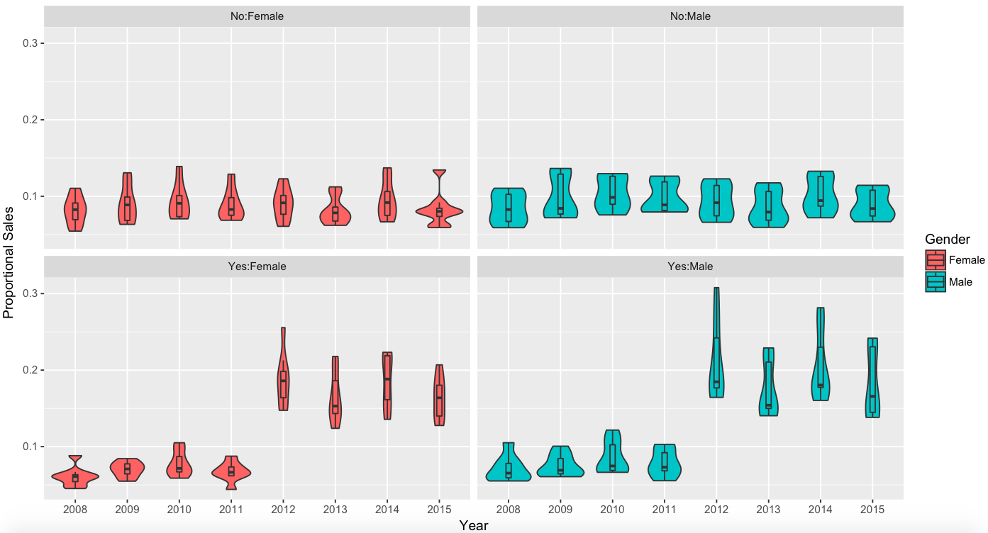
In the preliminary Explorative Data Analysis no outlier where found in the data set. From the comparative violin plot in Figure 1 , it clearly appears that yearly Proportional Sales does not depend on Gender but does depend on Training.

See Full Size >

Results of the Bayesian Statistical data analysis.

Instead of MCMC simulations, the INLA approach used in this study provides approximations to the posterior marginal distributions of the parameters. Summaries of these posterior distributions include posterior means and 95% Credible Intervals (CI), which play in Bayesian statistics the same role of the maximum likelihood estimates and 95% Confidence Intervals in classical Frequentist statistics.

The estimated distribution of the parameters of model1 are summarized as follows for each categorical covariate in the model: $Training$ (mean=0.364, 95% CI= [0.346,0.382]), $Gender$ (mean=0.079, 95% CI= [0.061,0.097]), $Age$ (mean=-0.021, 95% CI= [-0.025,-0.018]). Note that all CIs don’t contain 0. It means that all the related coefficients should be considered significantly different from 0. That is all covariates in model1 appears to be relevant drivers of Sales.

From the results of model2 fitting, only the CI related to $Training$ does not contain 0 (mean=0.426, 95% CI= [0.260,0.591]), that is $Training$ is the only significant driver of Sales.

In model comparison, $model2$ (DIC=4619.337, WAIC=5038.290) appears to be better than $model1$ (DIC=6468.970, WAIC=6673.552).

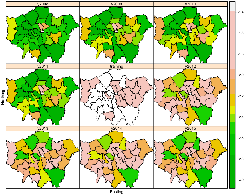
Maps may be a very useful tools for representing areal data. In Figure 2 maps of model2 fitted values are shown for each year. In the middle map the white units are those whose manager has not adopted the new approach. The non white areal units are related to managers that followed the training programme and adopted the new approach. It is easy to find units in the maps with low performance (green area) in the first four years (2008-2011), whose sales manager didn’t adopted the programme and with low performance also in the following 4 years (2012-2015). There are also units that improved their performance from green to orange because the related manager followed the training programme and adopted the new approach. This kind of maps may be very effective in showing the impact of the training programme on each areal unit.

The estimated distribution of the parameters of model3 are summarized as follows for each covariate in the model: $MSB$ (mean=10.288, CI=[9.307,11.289]), $Training$ (mean=0.734, CI=[0.602,0.861]), $Interaction$ (mean=2.506, CI=[1.007,4.076]). Note that all CIs don’t contain 0.

See Full Size >

References

- Arcaya, M., Brewster, M., Zigler, C. & Subramanian, S.V. (2012). Area variation in health: A spatial multilevel modeling approach. Health and Place, 18, 24-31.
- Bakka, H., Rue, H., Fuglstad, G.A., Riebler, A., Bolin, D., Illian, J., … Lindgren, F. (2018). Spatial Modelling with R-INLA: a Review. WIREs Computational Statistics, 10, 1-24. https://dx.doi.org/10.1002/wics.1443.
- Besag, J., York, J. & Mollie, A. (1991). Bayesian image restoration, with two applications in spatial statistics. Annals of the Institute of Statistical Mathematics, 43, 1-59.
- Besag, J. & Kooperg, C. (1995). On conditional and intrinsic autoregression. Biometrika, 82, 733-746.
- Bivand, R.S., Pebesma E. & Gomez-Rubio, V. (2013). Applied Spatial Data Analysis with R. (2nd ed.). New York, NY: Springer.
- Blangiardo, M. & Cameletti, M. (2015). Spatial and Spatio-temporal Bayesian Models with R-INLA. Chichester, UK: John Wiley & Sons.
- Congdon, P. (2017). Quantile Regression for Area Disease Counts: Bayesian Estimation using Generalized Poisson Regression. International Journal of Statistics in Medical Research, 6, 92-103.
- Cressie, N. (1993). Statistics for Spatial Data. New York, NY: Wiley.
- Dong., G., Ma, J., Harris, R. & Pryce, G. (2016). Spatial Random Slope Multilevel Modeling Using Multivariate Conditional Autoregressive Models: A Case Study of Subjective Travel Satisfaction in Beijing. Annals of the American Association of Geographers, 106(1), 19-35.
- Edwards, M.R. and Edwards, K. (2016). Predictive HR Analytics: Mastering the HR Metric. London, UK: Kogan Page.
- Elliott, P., Wakefield, J., Best, N. & Briggs, D., (Eds.). (2000). Spatial Epidemiology: Methods and Applications. Oxford University Press.
- Fitz-enz, J., & Mattox II, J.R. (2014). Predictive Analytics for Human Resources. New York, NY: Wiley.
- Gelman, A., Carlin, J.B., Stern, H.S., Dunson, D.B., Vehtari, A. & Rubin, D.B. (2013). Bayesian Data Analysis (3rd ed.). Boca Raton, FL: Chapman & Hall/CRC.
- Lee, D., Rushworth, A. & Napier, G. (2018). Spatio-Temporal Areal Unit Modeling in R with Conditional Autoregressive Priors Using the CARBayesST Package. Journal of Statistical Software, 84(9), 1-39.
- Lesaffre, E. & Lawson, A. (2012). Bayesian Biostatistics. Chichester, UK: John Wiley & Sons.
- Marr, B. (2018). Data-driven HR. New York, NY: Kogan Page.
- McCullagh, P. & Nelder, J. (1989). Generalized Linear Models (2nd ed). London: Chapman & Hall.
- R Core Team. (2017). R: A language and environment for statistical computing. R Foundation for Statistical Computing, Vienna, Austria. http://www.R-project.org/.
- Rue, H., Martino, S. & Chopin, N. (2009). Approximate Bayesian inference for latent Gaussian models using integrated nested Laplace approximations. Journal of the Royal Statistical Society: Series B, 71(2), 319-392.
- Rue, H., Riebler, A., Sørbye, S.H., Illian, J.B., Simpson, D.P. & Lindgren, F. (2017). Bayesian computing with INLA: a review. Annual Review of Statistics and Its Application, 4, 395-421.
- Sesil, J.C., (2013). Applying Advanced Analytics to HR Management Decision: Methods for selection, developing incentives and improving collaboration. Upper Saddle River, NJ: Pearson.
- Spiegelhalter, D.J., Best, N.G., Carlin, B.P. & Van der Linde, A. (2002). Bayesian measures of model complexity and fit (with discussion). Journal of the Royal Statistical Society, Series B, 64, 583-639.
- Wang, X., Yue, Y.R. & Faraway, J.J. (2018). Bayesian Regression Modeling with INLA. Boca Raton, FL: Chapman & Hall/CRC.
- Watanabe, S. (2010). Asymptotic equivalence of Bayes cross validation and widely applicable information criterion in singular learning theory. Journal of machine Learning Research. 11, 3571-3594.
- Wickham, H. (2016). ggplot2: Elegant graphics for data analysis. (2nd ed). New York, NY: Springer.
Copyright information
This work is licensed under a Creative Commons Attribution-NonCommercial-NoDerivatives 4.0 International License.
About this article
Publication Date
28 January 2019
Article Doi
eBook ISBN
978-1-80296-053-2
Publisher
Future Academy
Volume
54
Print ISBN (optional)
-
Edition Number
1st Edition
Pages
1-884
Subjects
Business, Innovation, Strategic management, Leadership, Technology, Sustainability
Cite this article as:
Giosa, M. D. (2019). Evaluating A Program On Hr With Spatially Structured Performance Data. In M. Özşahin, & T. Hıdırlar (Eds.), New Challenges in Leadership and Technology Management, vol 54. European Proceedings of Social and Behavioural Sciences (pp. 719-726). Future Academy. https://doi.org/10.15405/epsbs.2019.01.02.61