Education, Labour Market Status and Household Income Dynamics in Romania

Abstract

During the last decade Romania experienced considerable economic and social instability and household income has been subject to changes both in level and structure, though not equally for all households. It seems that low income households are more exposed to the risk of losing parts of their income during economic downturn, but also middle or high income households may be affected. Household characteristics, such as education and labour market status, are amongst the main determinants of household income level and can be associated with income dynamics. This paper aims at studying the role played by education and labour market status in the dynamics of household income in Romania in the period between 2007 and 2010. Our approach is twofold; we study the distribution and the income mobility patterns over time between income classes, paying attention to education and labour market status of household members. We attempt to analyse the extent to which education and labour market status count for the evolution of household income. A special focus has been on low income households. We base our analysis on EU-SILC data and we employ growth incidence curve analysis and transition matrices to determine the movement of households along the income distribution. Our results show that income dynamics is strongly related to education, as almost two thirds of the low income households are poorly educated and remain trapped in the same relative position on the income distribution over the years. Precarious labour market attachment as well is a drawback in income mobility.

Keywords: Income dynamicsincome mobilityeducationlabour market statuslow income households

1.Introduction

When the economic crisis of 2008 was beginning to show up, Romania was in the middle of a

flourishing economic period, with average income growth for all categories of population,

accompanied though by increases of income inequalities. Afterwards, during early crisis, household

income has declined on average and the income distribution has become more equalitarian in 2010 than

it used to be in 2007. Low income households have benefited more from growth (in 2007 and 2008)

and have lost less during the economic crisis than the rest of the households. The income dynamics has

been driven not solely by the developments of the market income levels, but also by the profound

changes in the tax-benefit system, which have been affecting the income distribution especially after

2010 along with the deepening of the crisis.

This paper attempts to study the developments regarding income distribution in the period between

2007 and 2010, focussing on household characteristics and income mobility. Our aim is the

investigation of the role played by education and labour market status in the income dynamics and

income mobility patterns of households. We base our analysis on the presumption that certain

households persist in having low levels of income irrespective of the overall developments (economic

growth or decline) and that we can identify these households by characteristics such as education and

labour market status which determine their income behaviour.

The rest of the paper is structured as follows. After a brief review of the previous empirical findings

regarding household income dynamics in Romania, we shall continue with the description of the

distributional effects of income growth, based on the growth incidence curves approach and the

identification of households at the bottom of the income distribution following education and labour

market status, in the second section. The next section deepens the longitudinal perspective and we

study a panel of households along the four year span and discuss on the educational and labour market

status of households who chronically remain at the bottom of the income distribution. The paper ends

with some concluding remarks.

2.Empirical Findings on the Developments of Income Distribution in Romania

Previous studies regarding income distribution in Romania have been extensively concentrated on

the analysis of income inequalities. For example, Precupetu (Precupetu & Precupetu, 2013) has

examined the dynamics of income inequalities in post-communist Romania (after 1990) and studied the

social impact of income inequalities and the effectiveness of social policies in combating inequalities.

Molnar (2010) has focused on the calculation and analysis of income inequality indices and has

decomposed inequality in between-group and within group components, by groups of main household

characteristics, showing that education and labour market status are the most important factors driving

between group inequalities. Zamfir et al. (2010: 58-75) have studied the impact of remittances sent

back from Romanians working abroad on income inequalities, overall and between urban and rural

areas, and they have shown that remittances were conducive to inequality reduction both between and

within rural and urban areas. Militaru and Stroe (2010) have investigated, following a growth incidence

curve approach, the income dynamics in Romania between 2000 and 2007, concluding that the economic growth which characterized the country’s development during those times was beneficial for the poor. The regional distribution of income has been analysed by Dachin and Mosora (2012) who pointed out that the employment structure of regions and the prevalence of subsistence agriculture shape the distribution of household incomes by regions. The effects of the economic crisis on income distribution in the rural areas have been investigated by Dachin and Sercin (2012) and revealed that household income in rural areas is less reactive to crisis than compared to the urban area. The economic mobility of households is strongly associated with the educational attainment of the household members, as Militaru et al. (2012) have substantiated through their analysis on mobility of households between income quantile groups, which shows that education is protective against downward income mobility and favours upward income mobility.

Income Dynamics and Household Characteristics, 2007-2010

Income dynamics

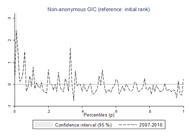
Methodology and data The distributional effects of growth between 2007 and 2010 have been examined using the growth incidence curves (GIC) approach (Ravallion & Chen, 2003; Bourguignon, 2010; Palmisano & van de Gaer, 2013). These curves basically compare the pre and post growth income distribution, by estimating the mean income growth against income quantiles and one can judge based on the shape of the curves whether the income growth between two points in time was more beneficial for certain parts of the income distribution. Because it is important to know if the low income state is chronic and what are the household characteristics that profile this persistent low income group, we have chosen to plot the non-anonymous GIC, which takes into account the joint distribution of initial and terminal incomes, or the initial income and the income change (Bourguignon, 2010). Individuals or households are ordered according to their initial income quantile p(yt-1) and we compute the quantile specific mean incomes growth rates, each quantile comprising the same individuals/ households in t as in t-1 (Grimm, 2005).

See Full Size >

where gt(p(yt-1)) is the mean income growth of the individuals/ households initially in the pth quantile, yt(p(yt-1)) is the income of the individuals/ households initially in the pth quantile at t and yt-1(p(yt-1)) is the income of the pth quantile at t-1. The data we use for growth incidence curve analysis is EU-SILC survey data (European Union Survey on Income and Living Conditions) for Romania. We have used the longitudinal component of the EU-SILC for Romania, the four year panel sub-sample (2008-2011, approx. 1850 households). The income reference data for EU-SILC is the calendar year before the data collection, therefore we have analysed 2007 to 2010 incomes. The household income is equivalised following the modified OECD equivalence scale to account for household size and composition. As a measure of living standard we

have used the household disposable income, which comprises all market income plus social transfers,

net of taxes and social contributions. Household income is expressed in constant prices of 2007, and

the bottom and top 1% of the sample were dropped in order to eliminate outliers (Palmisano, van de

Gaer, 2013).

Results

A general observation is concerning the fact that the mean household disposable income has

dropped by approximately 17% (real change, in 2007 constant prices) from 2007 to 2010, the economic

crisis affecting roughly all households. The pattern of the non-anonymous growth incidence curve,

which plots the income change taking into account the initial economic condition of the individuals,

appears progressive, as the bottom of the income distribution has lost less than the rest of the

distribution and below the mean income loss estimated for all households. The curve is clearly positive

for the bottom 10%, around zero for the rest of the distribution up to the 80%, and negative for the top

20% of the income distribution. In other words, the initially poor gain some income between 2007 and

2010, while the initially rich lose proportions of their income and the individuals initially located at the

middle of the distribution as well (see Fig. 1 ).

See Full Size >

Income Distribution and Household Characteristics

The role that household characteristics play in shaping the income distribution has been investigated

through the study of characteristics by income quintiles. This means that households were ordered

ascendingly by their disposable income and then, the so constructed distribution has been divided

equally in five groups, each comprising 20% of all the households. The poorest 20% of the households are found in the 1st quintile, and so on, the richest 20% of the households are positioned in the 5thquintile. Our focus shall be oriented towards the 1st and 2nd quintiles, in other words, the bottom 40% of

the income distribution. As we have mentioned before, we have paid attention to the following

dimensions: educational attainment of household members and labour market status of the household

members. We have based our analysis on EU-SILC data, the longitudinal component for the years

2008, 2009, 2010 and 2011, as described earlier in section 3 .1. Income reference period is one calendar

year before data collection, thus data on labour market status and education do not correspond to the

income period. Therefore, we have estimated the labour market status during income reference period

by the main monthly activity status, assuming that the status that has occurred most frequently during

the twelve months has been the main activity status for the entire year. The education variable is

collected for the current period and we assumed that it did not change since the income reference

period.

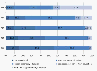
Education

As it can be seen in the figure below (Fig. 2), most of the household members from the bottom 40% of the income distribution (1st & 2nd quintile) have upper secondary or lower secondary education. At

the top of the income distribution (top 40%), still upper secondary education prevails, but tertiary

education gains grounds.

See Full Size >

The labour market attachment of the household members is, alongside education, the most important

determinant of the income level. We have investigated the distribution of households by the labour

market status of the household members and quintile groups based on equivalised household disposable

income (see Table 1 ). Only for the bottom 40% of the households, more than 10% of the household

members are self-employed or family workers, while the share of employees is well below the middle

and top quintiles. The share of inactive people, i.e. fulfilling domestic tasks and caring responsibilities,

disabled or/ and unfit to work, etc. is also considerable at the bottom 40%, almost 16% for the bottom

20% and 11% for the rest (20%-40%). We should mention that in Romania, self-employment and

especially self-employment in agriculture provides merely a subsistence living and stands for the most

widespread form of informal employment, with low compliance to social insurance schemes and

income tax evasion.

See Full Size >

The results for 2007, 2008 and 2009 show similar distributions as the above 2010 data, no

remarkable departure from this pattern is visible.

4.Economic Mobility, Education and Labour Market Status

Methodology and Data

We complement our income analysis with a longitudinal perspective on income dynamics, tracking

the same set of households throughout a four year time period. We are interested in the investigation of

the positional mobility of a household/individual’s income over time throughout the income

distribution. The arguments in favour of income mobility are numerous and the extent to which income

mobility is socially desirable highly depends on how this multi-faceted concept is defined (Jantti &

Jenkins, 2013). A higher degree of income mobility could be favourable for long-term inequality

reduction, but it could at the same time increase income risks, as income flows could become instable.

In the framework of equality of opportunity, a weak association with the original income, meaning that

each individual has the same chances of becoming rich regardless of his initial income level, is

beneficial (Peragine, Palmisano & Brunori, 2013). In this paper, we shall treat solely the issue of intra-

generational mobility, following a representative panel of Romanian households between 2007 and

2010.

A considerable amount of studies on income mobility relies on the traditional approach of

constructing transition matrices which are useful tools for summarizing the mobility content of

distributional transformations (Fields & Ok, 1999). The main disadvantage of using transition matrices

is that they neglect the individual income variations that take place within a specified income group.

However, our conclusions will complement those already drawn in the previous section concerning the

mobility profile investigated by means of non-anonymous income growth incidence curves.

Income mobility is assessed through the movement of households along the income distribution

which is divided into quintiles based on household income, equivalised following the modified OECD

scale, so each individual in a household has the same income (the equivalised income of the

household). We construct the transition matrices by computing the discrete Markov transitions

probabilities between time t and t+Δt : P , as the maximum likelihood estimator for the probability of

moving from state i to state j , thus pi,j= yi,j/yi , where yi,j is the total number of transitions from state i to state j over the time Δt and yi is the total number of individuals found in state i at the previous moment t . The space of states is defined by the income quintile groups.

Following the frame of our paper which concentrates on the bottom 40% of the income distribution,

we calculate bottom 40% entry and exit rates, i.e. the proportion of individuals who were initially (at t )

outside (in) the poorest 40% group and moved to (out) of this group (after Δt ).

In order to have a synthetic assessment of mobility as a summary of all individual transitions rather

than of those who are in a certain income group, we have calculated the Shorrocks mobility index (1978)

based on transition matrices as: M=[n-trace(Pi,j)]/(n-1) , where Pi,j is the transition matrix, the trace (Pij) is the sum of the elements of the main diagonal of Pi,j and n is the number of income groups. We have calculated the mobility index for each of the one year transitions and examined its changes in time.

We use EU-SILC longitudinal component data collected from 2008 to 2011, with income reference years from 2007 to 2010. We analyse the sample (approx. 1850 households) which is common for all four years; therefore we are able to calculate the one year transition matrices and the three year transition matrix as well. The sample is representative for the entire population. The results are presented below.

4.1.Main Findings

The transition matrices calculated based on household disposable income (see Table 2 ) show that

there is a persistency at the bottom of the income distribution, as households who were in the bottom

40% of the income distribution at the initial moment, are more likely to be in the same relative position

after one year. More than two thirds of the households remain in low income groups from one year to

another. However, the mobility pattern has changed in time. Between 2007 and 2008 when Romania

has not yet been hit by the economic crisis, the income mobility not only of lower quintiles was higher

than compared to the years to come. The mobility is particularly visible between neighbour income

groups.

During crisis, most of the households preserve their relative positioning throughout the income

distribution, in spite that the poorer households gain some income, while the rich part of the

distribution loses some fraction of its income.

See Full Size >

The overall mobility index ranges from 0.46 for 2007-2008 to 0.28 for 2009-2010, pointing towards

a less intense movement between income groups in times of crisis. The same idea particularized to the

bottom 40% income group comes from the examination of exit and entry rates from and into this

income group. So, the exit as well as the entry rate to this group decrease in crisis (see Table 3 ).

However, throughout the entire period under analysis, 23.8 % of those who were initially (in 2007) in

the low income quintiles have managed to exit by 2010 towards higher income groups and 13.4% of

those who initially were not belonging to the poorest income group eventually fell into this category.

See Full Size >

If we look at the picture of overall movements between 2007 and 2010 (see Table 4 below), it seems that 62.1% of the households who were in 2007 in the 1st quintile, were still at the very bottom of the distribution in 2010. Nevertheless, almost one third of them succeeded in moving to the 2nd quintile and around 8% to the middle quintile. As we have previously seen, in their case, the level of income generally increased slightly during these years. The 2nd quintile households were not benefiting of income growth, they actually have preserved their real income, and therefore almost 20% of them switched their position in the income distribution with households who were initially in the 1st quintile.

See Full Size >

As we have seen, for a considerable proportion of households, persistency at the bottom of the income distribution is a common fact. We have also investigated the characteristics of these households who have chronically remained at the bottom, regardless of the economic developments that took place (economic growth in 2007 and 2008 and economic decline in 2009 and 2010). As it is shown in the figure below (Fig. 3), low education is a characteristic of around 70% of the households that persist in the 1st quintile.

See Full Size >

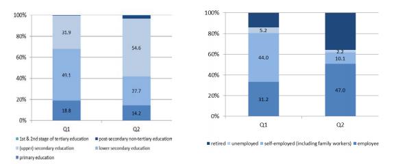
Approximately half of the households that have been trapped in the 2nd quintile have at most lower

secondary education. The relationship with the labour market is precarious for more than 50% of the

households who were at the very bottom of the income distribution between 2007 and 2010. Most of

the adult members of these households are self-employed or family workers, particularly in agricultural

activities, being trapped in an unproductive and often informal employment. Informality is a survival

strategy for most of those who work as self-employed or unpaid family workers in agriculture, and they gather the majority of the informal workers in Romania. The 2nd quintile group’s composition is completely different, as almost half of the adult household members are employees and one third are retired. The introduction of a minimum social assistance pension in 2009 has improved to some extent the living standard of pensioners, thus the likelihood of finding them in the 1st quintile has lowered. The analysis is conditional on the labour market status during the first year of analysis; in the following years, the most remarkable changes in the individuals’ status concern the transition from employment to unemployment, as a consequence of decreasing labour demand during the economic crisis.

It seems that the households trapped at the bottom perform (with respect to the characteristics mentioned above) worse off than the average of all households at the bottom for each year. This is to say that better education and a closer relationship with the labour market significantly increase the mobility chances of a household on the income ladder.

5.Concluding Remarks

The study has focused on the investigation of income dynamics in Romania, its aim being that of

giving a description of the distributional changes in household income levels and of exploring the main

characteristics of the households in relation to their income dynamics. We have focused on

characteristics such as education and labour market status of household members in order to investigate

whether there can be established a link between these variables and income immobility and persistency

at the bottom of the income distribution.

Our results have shown that for the period between 2007 and 2010, the disposable income at

household level has dropped for almost all households. Conditional on the initial ranking of the

households in the non-anonymous growth incidence analysis framework, the examination of income

dynamics shows that the initially poor have slightly increased their disposable income, while the

initially rich lost fractions of their income.

We have given a special attention to the bottom of the income distribution and compared these

households with those from the middle and top of the distribution with respect to some household

characteristics that are generally conducive to low levels of income. Not surprisingly, low education

and weak labour market attachment (vulnerable employment, informal employment, and inactivity) are

the main differentiating features between bottom 40% households and the rest. The analysis has also revealed the fact that the bottom 40% group is not homogeneous, as the 1st quintile group differs to some extent in certain dimensions from the 2nd quintile group. There are striking similarities from one year to another, meaning that the households at the bottom of the income distribution hold roughly the same characteristics each year.

We have tracked the same set of households along the four year time span (2007-2010). The traditional approach of transition matrices between income groups has been employed in order to assess the positional mobility of the households on the income distribution. We have observed higher income mobility in the pre-crisis year (2008) and an increased immobility in the years of economic crisis, when the entry and exit rates from the lowest 40% income group have dropped. More than 60% of the 1st quintile group households and almost half of the 2nd quintile group households are trapped in the same position for four years. It is clear that their educational attainment and their links with the labour market are more precarious than of the households that are transitory at the very bottom.

Acknowledgement

The results presented in this paper are part of the study conducted by the author for the World Bank Project: Shared Prosperity in the EU11.

References

1. Bourguignon, F. (2010). Non-anonymous Growth Incidence Curves, Income Mobility and Social Welfare Dominance: a theoretical framework with an application to the Global Economy. G-MonD, Working Paper no.14.
2. Dachin, A., Mosora, L.C. (2012). Influence factors of regional household income disparities in Romania. Journal of Social and Economic Statistics, 1(1), Summer 2012.
3. Dachin, A., Sercin, A. (2012). Effects of the economic crisis on rural household incomes in Romania. Paper presented at the 3rd International Symposium "Agrarian Economy and Rural Development - realities and perspectives for Romania", Bucharest, Romania.
4. Fields, G., Ok, E.A. (1999). The Measurement of Income Mobility: An Introduction to the Literature. Cornell University ILR Collection.
5. Grimm, M. (2005). Removing the anonymity axiom in assessing pro-poor growth. Ibero-America Institute for Economic Research Discussion Paper No. 133.
6. Jantti, M., Jenkins, S.P. (2013). Income mobility. IZA DP no. 7730, Discussion Paper Series.
7. Militaru, E., Stroe, C. (2010). Poverty and Income Growth: Measuring Pro-Poor Growth in the Case of Romania. Proceedings of the 11th WSEAS Mathematics and Computers in Science Engineering, WSEAS Press.
8. Militaru, E., Zamfir, A.M., Mocanu, C., Lungu, E.O. (2012). Does education influence income mobility in Romania? paper presented at the NTTS 2013 Conference.
9. Molnar, M. (2010). Income distribution in Romania. MPRA Paper No. 30062.
10. Palmisano, F., van de Gaer, D. (2013). History dependent growth incidence: A characterisation and an application to the economic crisis in Italy. ECINEQ WP 2013 – 314.
11. Peragine, V., Palmisano, F., Brunori, P. (2013). Economic Growth and Equality of Opportunity. Policy Research Working Paper 6599, The World Bank.
12. Precupetu, I., Precupetu, M. (2013). Growing inequalities and their impacts in Romania. Country Report, GINI Growing inequalities’ impact.
13. Ravallion, M., Chen, S. (2003). Measuring Pro-Poor Growth. Economics Letters, 78(1), 93-99.
14. Zamfir, A. M., Mocanu, C., Militaru, E., Pîrciog, S. (2010). Impact of Remittances on Income Inequalities in Romania. In U. Schuerkens, ed., Globalization and Transformations of Social Inequality, London: Routledge Taylor& Francis Group.