Does Social Mobility Effect Poverty?

Abstract

This study attempts to investigate the intergenerational social mobility in Malaysia by focusing on the phenomenon of rural people getting out of the poverty circle. The analysis is based on a survey of the rural households in the northern region of Malaysia, comprising the states of Kedah, Perlis, Pulau Pinang and Perak. The impact of social mobility on poverty is analyzed using logit model where nine independent variables are used. The dependent variable which is the level of education of the son is used as a proxy to determine whether the person is poor or not. Those sons who achieved lower than a diploma is categorised as poor. Meanwhile, social mobility is categorised into four, namely no mobility, low mobility, medium mobility and high mobility. Our findings show that there are only four factors (mobility, asset ownership, the existence of a university in the near vicinity and the respondents’ house being near to town)that significantly affect poverty among the children. We found that the higher the social mobility, the lower the poverty.

Keywords: Povertysocial mobility

Introduction

This study presents a comprehensive attempt to investigate the intergenerational social mobility in Malaysia by focusing on the phenomenon of rural people getting out of the poverty circle. Intergenerational social mobility can be measured in several ways, by income, education, occupation or social class. More often, economic research has focused on some measure of income or wages. Normaly, household’s disposable income is used to measure the standard of living of individuals (Chadwick, & Solon, 2002; Solon, 2004; Lee, & Solon, 2006). In practice, accurate measurement of a household’s disposable income is difficult because the structure of the household it self. Therefore, most existing studies use some measure of wages.

There are a variety of public and private development projects in the rural areas. Educational institutions such as primary schools, secondary schools, colleges, and universities sprouted conspicuously as well as infrastructure facilities such as roads, airports enlarged and upgraded as an international airport and so on. These things are the new engine of growth in the rural communities.

However, what is the position of the rural communities today compared to ten or fifteen years ago? Have their families escaped the cycle of poverty and backwardness?

As we all know, education is an important factor to bring change. Education is one of the highest dimensions of the Malays to experience mobility since colonial times until today. Educational achievement can determine whether a person will follow in their father’s footstep as farmers and labourers or secures high positions in public administration or private sector.

Literature Review

Azevedo, & Cesar (2010) stated that while intergenerational education mobility have improved in recent decades, which may increase income mobility for younger cohorts, overall, the Latin American region still presents lower intergenerational social mobility. Previous studies suggest that these results might be associated to social exclusion, low access to higher education, public policies and labour market discrimination.

According to D’Addio (2007) parental background can influence their offspring’s wages in various ways. In very general terms, parental background can affect these wages by boosting both the offspring’s labour productivity and their successful insertion in the labour market. One way in which children’s productivity, and hence their future incomes, can be enhanced is through the ability of parents to invest in their offspring’s human capital. (Eberharter, 2013) used data from the German Socio-Economic Panel (SOEP), the Panel Study of Income Dynamics (PSID), and the British Household Panel Survey (BHPS) to analyse the hypotheses that the extent and the determinants of intergenerational income mobility and the relative risk of poverty differ with respect to the existing welfare state regime, family role patterns, and social policy design. The empirical results indicate a higher intergenerational income elasticity in the United States than in Germany and Great Britain, country differences concerning the influence of individual and parental socio-economic characteristics, and social exclusion attributes on intergenerational income mobility and the relative risk of poverty.

Causa & Johansson (2010) wrote that early childcare and education play a role in explaining observed differences in intergenerational social mobility across countries. In addition, their study also found a positive cross-country correlation between intergenerational social mobility and redistributive policies.

Causa & Johansson (2009) examines the potential role of public policies and labour and product market institutions in explaining observed differences in intergenerational wage mobility across 14 European OECD countries. Their empirical results show that education is one important driver of intergenerational wage persistence across European countries. There is a positive cross-country correlation between intergenerational wage mobility and redistributive policies, as well as a positive correlation between wage-setting institutions that compress the wage distribution and mobility.

Methodology

This study involves four states in the north Peninsular Malaysia which are Perlis, Kedah, Penang and Perak. All respondents are located in the rural areas. The sampling frame was obtained from the Statistics Department, Kuala Lumpur. Though the originally given sample was 400, after undergoing data refining process, the total number suitable for analysis was only 333. All these respondents met the study criteria which is a father who is 50 years old and above and have at the very least one son who is working.

In this study, we used parental background by the highest educational qualification level achieved by the father as proxy. Education is likely to be a more permanent feature than current wages. The results focus on father (aged 50 and above) and their son/daughter (the child who has achieved the highest level of education in the family; hereafter called son).

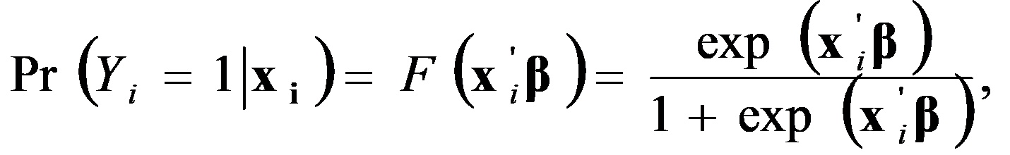
To analyze the effect of social mobility on the probability of occurrence of poverty we employ a binary choice model based on the maximum likelihood method. We used (0 and 1) as a dummy dependence variable. The son’s educational level variable is used as a proxy to determine whether the son is poor or the opposite. In particular, a son having tertiary education level (Diploma and above) is categorized as being not poor and is given the value one (1), whereas a son having a lower than diploma education level is categorized as being poor and given the value zero (0).

The logit model for this study:

Specification of latent variable:

Yi* = β Xi + ui (1)

where:

Yi = 1 (not poor) if Yi* > 0

Yi = 0 (poor) if Yi* ≤ 0

ui = error term

β = estimated parameter.

Xi = vector of independent variables

The probability of inter-generation i being poor or otherwise, is postulated to depend on nine independent variables which are Social Mobility (Social Mobility), Father attitude (Att_Father); Father involvement in the community (Inv_Community); Asset ownership in the family (Asset); Existence of a university near respondent’s house (Available_Uni); Distance from respondent’s house to town centre (Near_Town); Distance of respondent’s house to highway (Near_highway); Distance from respondent’s house to bus station (Near Bus Station) and Position of the respondent’s house with tourism centre ( Near_Tourism_Loc).

See Full Size >

where

xi’= [Social MobilityiAtt_FatheriInv_CommunityiAssetiAvaiable_UniiNear_TowniNear_highwayi Near Bus Stationi]

Equation (2) is used to estimate the probability of not poor among the respondent. Whether the independent variable has a positive or negative impact on the dependent variable is depend on the sign of the estimated parameter (Wooldridge, 2002). Other than that, the odds ratio used to examined the impact of the independent variables on the dependent variable. With the value of the independent variables, the estimated value for the dependent variable could be interpreted as the probability of the respondent not poor (Greene, 2006; Long, Scott, & Jeremy, 2006; Maddala, 1983)

In order to study the effect of social mobility on the probability of occurrence of poverty, the son’s educational level variable is used as a proxy to determine whether the son is poor or the opposite. In particular, a son having tertiary education level (Diploma and above) is categorized as being not poor and is given the value one (1), whereas a son having a lower than diploma education level is categorized as being poor and given the value zero (0).

Social mobility variable is included as the main variable to be studied in influencing the probability of occurrence of poverty among the respondents’ son. Social mobility is divided into four category which are no mobility, low mobility, medium-high mobility and high mobility. No mobility means that there is no change in the educational achievement between the respondent and his son. As an example, if a respondent has PMR education level and his son also has the same education level, the conclusion is there has been no social mobility for this respondent. Nonetheless, for a respondent who is currently at the tertiary education level and having a son also at the tertiary level, even though there is no change is social mobility, this study considers him to have social mobility, that is high level social mobility.

In contrast, low level mobility category is a change of one educational level between a respondent and his son whereas medium-high level social mobility shows there has been a change of two educational level between the respondent (father) and his son. Next, high level social mobility exists when there are larger changes, that is more than two educational level between father and son.

Finding

The area studied is the rural areas in these four states, namely Perak, Kedah, Perlis and Pulau Pinang. Perak has the highest number of respondents with 151 respondents (45 per cent). This is followed by the states of Kedah with 138 respondents (41 per cent), Perlis and Pulau Pinang which recorded 7 per cent of respondents each. This field study data was obtained starting from early 2015. The rural communities selected as respondents are the head of the family, that is fathers aged 50 years and older and having a son who works aged 25 years or older. A total of 333 people from the rural communities were selected based on the selection made by the Department of Statistics Malaysia.

Table 1 shows information about the formal education possessed by the respondents who are fathers and the respondents’ son. The level of formal education is divided into four classifications, which are no schooling, primary school, lower secondary school (SRP/PMR), higher secondary school (SPM), tertiary education (diploma/degree).

This study examines the highest level of formal education attained between two generations, that is, the education level of parents and children. As shown in Table 1 , the level of educational attainment by two generations, that is between parents (the new era of independence) and child (around 25-30 years earlier) shows a significant improvement. In accordance with the life in the new era of independence with rampant deprivation and limited access to education, 32.1 per cent of the fathers have never received any formal education. Moreover, only 67.9 per cent of the fathers have gone through a formal education system where 39 per cent have attained secondary education level and 1.5 per cent have tertiary education.

There is a noticeable increase in the level of education obtained by the sons where almost 100 percent of them have received formal education. Moreover, only 0.3 percent have never received any formal education while 1.8 percent have received primary education. Almost 98 percent of them have secondary level of education and above. In fact, almost 40 percent of the son has received a tertiary education.

Generally, the study has found that there has been a transformation in terms of mobility in rural communities based on the educational aspect that is achieved by the two generations under study, the generations of parents and children. Mobility by level of education is recognized in importance as a key prerequisite for achieving a better life for the rural communities. This reflects that people have become more aware of the importance of formal education in life. In addition, through the well-organised national education system, rural people are able to obtain formal education.

Table 2 shows the impact of social mobility on poverty. In this analysis, the son’s level of education variable is used as a proxy for determining whether the son is poor or the opposite. In particular, a son who receives high- level education (Diploma and above) is classified as not poor and is given the value one (1), while a son who receives a level of education lower than a diploma is classified as poor and given the value zero (0).

In the analysis, social mobility is divided into four categories, namely no mobility, low mobility, medium-high mobility and high mobility. No mobility means there is no change in educational attainment between the respondent and his son. For example, if a respondent’s education level is at PMR and his son also has PMR level of education, then the conclusion is there has been no social mobility for the respondent. However, for respondents who are at high-level education and have a son also at high-level education, although this shows no change in social mobility, this study considers they have social mobility, namely high level social mobility.

Low mobility category is a change in one level of education between the respondents and their son. As an example, if a respondent (father) has an education level at PMR, but his son has an education level at SPM, then is categorized as respondent having low level social mobility.

Medium-high level social mobility exists when there is a change involving two levels of education between the respondent (father) and his son. As an example, if a respondent has an education level at PMR, but his son has an education at Diploma level, then this respondent is said to have medium-high social mobility.

On the other hand, high level social mobility occurs when there is a large change or involving more than two levels of education. As an example, if the respondent (father) has a primary school education, but his son has an education at the diploma level and above, then this respondent is said to have high level social mobility. High level social mobility also refers to the attainment of a level of education at the tertiary level by the son.

Social mobility factor shows a significant value at the 1% level in determining the probability that the son will turn out poor. The positive relationship shown means that the higher the social mobility level occurring between a father and son, then the higher the probability of the son to not become poor. The study found that the effect of a change in social mobility shown by the odds ratio in social mobility is 1,7690. This means that an increase in one social mobility level will cause the odds value for the probability of the son to not become poor increases by a factor of 1.77, ceteris paribus. This implies that if the same space and opportunity are given to an individual, the probability of that individual to become poor is low.

Conclusion

The impact of social mobility on poverty is analyzed using logit model where nine independent variables are used. The dependent variable which is the level of education of the son is used as a proxy to determine whether the person is poor or not. Those sons who attained high levels of education (which is diploma and above) are not categorized as poor. On the other hand, those who achieved lower than a diploma is categorised as poor. Meanwhile, social mobility is categorised into four, namely no mobility, low mobility, medium mobility and high mobility. Our findings show that there are only four factors that significantly affect poverty among the children. The four factors are social mobility, asset ownership, the existence of a university in the near vicinity and the respondents’ house being near to town.

References

1. Azevedo, V. M. R., & Cesar P. B. (2010). Intergenerational social mobility in Latin America: a review of existing evidence. Revista de Análisis Económico, 25 (2).
2. Causa, O. Dantan, S. & Johansson, A. (2009). Intergenerational social mobility in European OECD countries. OECD Economics Department Working Paper No. 709. OECD.
3. Causa, O. & Johansson, Å. (2010). Intergenerational social mobility in OECD countries. OECD Journal: Economic Studies.
4. Chadwick, L. & Solon, G. (2002). Intergenerational income mobility among daughters. The American Economic Review, 92 (1).
5. D’Addio, A.C. (2007). Intergenerational transmission of disadvantage: mobility or immobility across generations? A Review of the Evidence for OECD Countries, OECD Social, Employment and Migration Working Paper No. 52.
6. Eberharter, V.V. (2013). The intergenerational transmission of occupational preferences, segregation, and wage inequality – empirical evidence from Europe and the United States. Journal of Applied Social Science Studies, 133(2).
7. Greene, W. H. (2000). Econometric analysis. New Jersey:Prentice-Hall International, Inc.
8. Lee, Chuil-In. & Solon, G. (2006). Trends in intergenerational income mobility. NBER Working Papers 12007, National Bureau of Economic Research, Inc.
9. Long, J. Scott, F. & Jeremy, F. (2006). Regression model for categorical dependent variables using stata. Texas: Stata Press Publication Stata, Corp LP College Station.
10. Maddala, G.S. (1983). Limited-dependent and qualitative variables in econometrics. Cambridge: Cambridge University Press.
11. Solon, G. (2004). A model of intergenerational mobility variation over time and place. In Generational income mobility in North America and Europe, M. Corak (eds.), Cambridge University Press, Cambridge, England.
12. Wooldridge, J.M. (2002). Econometric analysis of cross section and panel data. Massachusetts: The MIT Press.