Pavement Roughness Modeling Using Regression And Ann Methods For Ltpp Western Region

Review of relevant literature

Road roughness in particular indicates ride quality of any road users (AASHO, 1962). The IRI was the current standard roughness indicator being used worldwide. Meegoda and Gao (2014) studied the time-sequence surface roughness data of the General Pavement Study (GPS) test sections and developed a model to predict surface roughness progression as the pavement age increases. The final model is shown in Equation 1.

$\ln {IRI}_{i+\mathrm{1}}-\ln {IRI}_i={\left({\alpha }_{i+\mathrm{1}}\mathrm{*}{t}_{i+\mathrm{1}}^{\mathrm{0.9715}}-{\alpha }_{i+\mathrm{1}}\mathrm{*}{t}_i^{\mathrm{0.9715}}\right)}_{.}$ Eq. 1

The alpha (α) describes the deterioration rate of the pavement as a function of cumulative traffic loads (KESALs/year), structural number (SN), freezing index (FI), and annual precipitation (AP). The General Pavement Study (GPS) 1 data sets from 13 states were used to validate the model. The reliability of the roughness progression of the asphalt pavements was modelled using the Weibull distribution. The results showed that the difference in the median roughness value between the measured and predicted values was not significant. There is no correlation coefficient, R value of the measured vs. estimated IRI plot was reported; however, the plot indicated that the data points fit closely to the equality line, which suggests a reliable model.

Madanat, Nakat, Farshidi, Sathaye, and Harvey (2005) developed a mathematical model to predict the progression of the asphalt pavement roughness. In this study, the linear regression equations were developed to predict increment of roughness progression (∆IRI) using Washington State’s Pavement Management System (PMS) database. Eight independent variables were used which include the IRI in previous year, ESAL changes in the year of observation, cumulative ESAL, base thickness, total asphalt layer thickness, time since last asphalt overlay or bituminous surface treatment (BST) overlay, minimum air temperature, and yearly precipitation. In addition, three dichotomous variables for asphalt overlay, BST overlay, and maintenance application were also considered. The linear regression’s R of 0.725 was observed; however, no R value of the measured vs. predicted IRI was reported.

Attoh-Okine (1994) applied the (Artificial Neural Network) ANN’s back-propagation method to evaluate the capabilities of the ANN to predict roughness progression in the flexible pavement. An extensive research investigated structural deformation as the factors of modified SN, increment of traffic loads, severity of cracking and thickness of cracked layer, and incremental variation of rut depth. Kargah-Ostadi, Stoffels, and Tabatabaee, (2010) developed the changes in IRI over time roughness prediction model for rehabilitation recommendation using the ANN. The statistical analysis on 20 variables was conducted to determine any significant correlation with IRI. Only eight variables were included in the final model. The R of 0.979 was observed which shows that it is feasible to use IRI as the prediction criteria.

Comparison of the Southern region enhanced regression equation with the AASHTO MEPDG equation

Mohamed Jaafar et al. (2015) developed the enhanced linear regression that incorporates dichotomous (dummy) variable for construction number, namely CND for the LTPP southern region test sections. Figure 1 illustrates the IRI values (both measured and predicted) for data sets in Southern Region. The improved regression equation was included in the plot and high R value of 0.865 between the measured and predicted IRI values was observed. The comparisons using the enhanced regression equation and the MEPDG model were conducted based on 10 independent data sets from 1990 to 1995 (FHWA 2009; MDOT, 2013).

See Full Size >

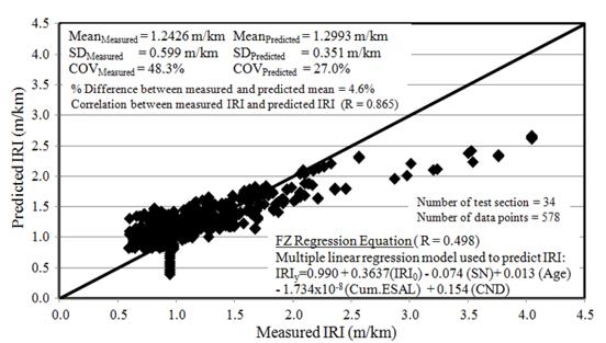
The overall results showed that the MEPDG forecasts are deprived for most of the data sets. The enhanced regression equation showed a better R of 0.874 compared to the predictions by the MEPDG regression equation (R is 0.819). In addition, the mean IRI values predicted by the MEPDG equation is about 23% higher than the measured IRI (mean value). The difference is greater compared to the enhanced equation’s prediction with only 5.5% more than the mean measured IRI value (Mohamed Jaafar et al., 2015). A similar approach was used to develop the enhanced dummy regression equation to assess the reliability of the equation to predict future IRI value in the Western region. However, no comparison with the MEPDG equation will be conducted since the rut depth data sets for GPS 2 in the Western region are missing completely, either from online LTPP database or LTPP standard data release 26.0 CDs.

Dependent variable

In the enhanced dummy regression equation, average yearly IRI (average IRI values for both left and right wheel path) is selected as the dependent variable. The IRI values are measured with a minimum of five runs for each side. The processed yearly IRI data indicate approximately 46% of the IRI data are excluded from the database. Thus, the following methods are implemented to interpolate the missing yearly IRI data:

• If the initial yearly IRI data are not available, the missing data are assigned with the same IRI value as the first measured IRI data. For example, the yearly IRI data in 1990 and 1991 are unavailable, and the first measured data is in 1992. Therefore, the IRI in 1990 and 1991 are assumed similar to the IRI value in 1992.
• If the yearly IRI data are missing after the final year of the measured IRI, the subsequent years will have the same IRI value as the final measured IRI data. For example, the final yearly IRI data in 2004 are available. Thus the yearly IRI data for 2005 and 2006 are assumed similar to the yearly IRI data in 2004.
• If the IRI data are missing in between two measured yearly IRI data, for example the IRI data are measured in 1990 and 1992, but not in 1991, then the IRI value in 1991 is the average of IRI value measured in 1990 and 1992.

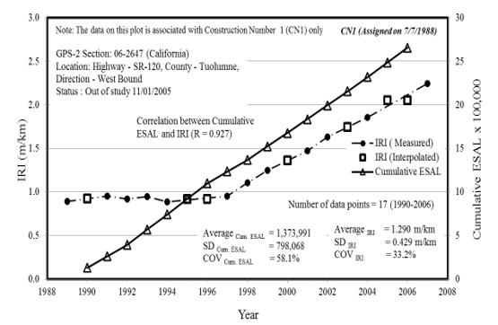
Figure 2 indicates the measured and interpolated IRI values for test section 06-2647 in the California, together with the cumulative ESAL traffic application data. A total of 17 data points are plotted and the IRI value in 1990 is interpolated by considering mean IRI value between 1989 and 1991. The IRI values for 1995 and 1996 are the average yearly IRI values between 1994 and 1997. If necessary, the yearly IRI value for 2008 is assumed similar to the yearly IRI in 2007. The ESAL data are the cumulative values of the total annual ESAL. The yearly IRI and the cumulative ESAL exhibit a strong correlation with R equal to 0.927.

See Full Size >

Independent variable

Four independent variables of IRI₀, cumulative ESAL, SN, and age are selected to develop the enhanced regression equation. Pre-processing of the yearly IRI data showed 48.5% of the annual ESAL traffic data are unavailable from the LTPP database. Therefore, the ESALs are determined based on the average annual rate of growth (AARG) concept (Mohamed Jaafar et al., 2015). The authors also described in detail each variable used in the prediction equations.

• Yearly IRI: The yearly IRI are between 0.319 m/km to 3.208 m/km, with an average value of 1.401 m/km. The Standard Deviation (SD) and Coefficient of Variation (COV) are 0.561 m/km, and 40.0%, respectively.
• The IRI0 has an average value of 1.274 m/km. The SD and COV are 0.374 m/km and 29.4%, respectively. The correlation between the yearly IRI and IRI0 was 0.464.
• Cumulative ESALs: The values range from 18,000 to 26,684,104 with an average value of 3,511,167. The SD and COV are 5,001,990 and 142.5%, respectively. The cumulative ESAL traffic and yearly IRI showed R value of -0.128. Cumulative ESAL data indicated higher variation as compared to the yearly IRI data.
• The average SN is 5.4 with the SD equal to 1.4. The calculated COV is approximately 26%. The SN ranged from 2.9 to 8.8. Repetitive traffic load impacts affected the IRI and structural capacity. A weak negative correlation between yearly IRI and SN (R = - 0.145) was observed. The IRI is relatively higher for a pavement structure with lower SN value.
• Pavement age: Range from three years (test section 56-7773, Wyoming in 1990) to 39 years (test section 06-7491, California in 2006) with an average value of 21 years. The SD and COV are both 7.5 years and 35.8%, respectively. The yearly IRI is positively correlates with pavement age with Pearson’s R equal to 0.197, which shows that the IRI increases with pavement age.

Description on the data used for IRI modeling in the Western region

• The data sets for 32 test sections are downloaded from the LTPP database and the IRI0 data are determined from the downloaded data sets.
• The IRI values from left and right wheel path from different runs are averaged and noted as yearly IRI. The missing yearly IRI data are determined as discussed in Figure 1. These statistics are computed for all test sections with IRI0 less than 2 m/km, except for the test sections 08-2008 and 08-7781, both at US 82 highway in Bent County, Colorado.
• A total of 32 LTPP test sections are analysed. The average IRI0 is 1.274 m/km with the SD of 0.374 m/km and the COV of 29.4%.
• The measured yearly IRI data from the database and the missing yearly IRI values estimated using AARG (Mohamed Jaafar et al., 2015) are considered in the analysis.

The example of the interpolated missing ESAL values and the annual cumulative ESALs are shown in Figure 3. Test section 06-2647 is in Tuolumne County, California. The interpolated annual ESAL showed constant increments, corresponding to positive AARG of 1.5%. A few test sections showed negative AARG values, resulted in the smaller interpolated traffic ESAL values.

See Full Size >

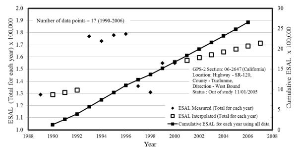
Table 1 shows the correlations between each of the variables. About 544 data sets are included (17 years x 32 test sections). The analysis discovered large variability in the yearly IRI data based on the COV value. The Pearson’s R, mean, SD, and COV values for IRI data shown are related to both measured and interpolated data.

The IRI₀, Age, SN, and Cumulative ESAL indicated statistically significant correlations with the yearly IRI. All variables showed statistically significant correlations except for SN with IRI₀ and SN with cumulative ESAL, respectively with p-value more than 0.05. In addition, the observed R values are less than 0.1. This resulted in no significant correlations between the variables. There are some variations in each variable depicted by COV less or equal to 40%. The exception is the cumulative ESAL with COV of about 142.5%, showing large variation in traffic volume data. Higher variation in the data sets will produce a better enhanced dummy regression equation.

Description on the construction number for the test section 041065 in Arizona

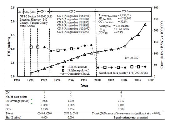
Previously, Figure 1 described the yearly IRI time series data for only one test section with original construction number (CN1). The yearly IRI value consistently increase every year except a slight decrease observed in 1992 and 1994. Commonly, majority of the test sections had more than one CN value. Only seven test sections remained at CN1. The remaining 25 test sections indicated more than one CN values. Four test sections recorded CN1 to CN6 (04-1065, 06-2002, 06-2040, and 56-5772). As an illustration, Figure 4 shows multiple CN values for section 041065, located at Interstate 40, in Yavapai County, Arizona. This test section recorded up to six construction numbers which as shown in Figure 4 plot. The vertical lines describe the year of each assigned CN value. For this test section, CN2 to CN3 were assigned after a local maintenance to patch the potholes was completed. In addition, CN4 and CN5 were assigned after the major maintenance of grinding, milling and surface overlay. These maintenance applications improved the road condition with smoother surfaces, thus reducing observed the IRI values. The IRI values at each subsequent CN decrease sharply as seen in CN5 and CN6 years. The yearly IRI values increase again until the subsequence maintenance and rehabilitation year. The yearly IRI and cumulative ESAL time series plot showed a strong correlation with R equal to -0.749.

See Full Size >

Artificial Neural Network Modeling of IRI

The static, feedback, and dynamic ANN analysis was conducted to develop the ANN roughness prediction models. The static ANN is the simplest and the most widely used network. It is a multi-layered feed-forward neural network that is trained using an error-backpropagation algorithm (Najjar, 1990). In the analysis, the best network performance was achieved after 20,000 training iterations on all training data sets. The feedback ANN is like the static ANN, except an additional independent variable was introduced. The new independent variable is the predicted IRI values from the static ANN. The dynamic ANN involves sequential analysis of each data set. For this sequential analysis purposes, each data set was duplicated five times using Visual Basic for Application (VBA) codes in Microsoft Excel (Yasarer, 2013). Once the dynamic ANN analysis was completed, only the predicted IRI values from the fifth data sets for each test section were considered for comparison purposes.

Verification of the enhanced dummy regression equation for the Western region

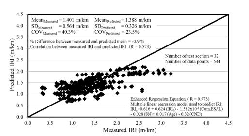
Figure 5 shows the predicted and measured IRI values for all 544 data points associated with 32 LTPP’s GPS 2 test sections used to develop enhanced dummy regression equation. The R of 0.573 is observed between the measured and predicted IRI values. The difference between the mean predicted IRI and the mean measured IRI is -0.9%. Therefore, the enhanced dummy regression equation fits the data reasonably well. A total of 39 measured IRI data sets from 20 test sections are verified with the predictions from the enhanced dummy regression equation as shown in Figure 6.

See Full Size >

See Full Size >

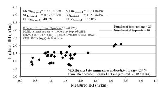
The correlation between the measured and predicted IRI is 0.564. The difference between the mean of the predicted and measured IRI is -2.9%. The enhanced dummy regression equation works considerably well for the GPS 2 test sections in the Western region. The measured and predicted mean IRI values are approximately the same but the predicted values show less variation.

Static, feedback, and dynamic ANN models

In developing the desired ANN models, the static and feedback ANN adopted similar number of training, testing, validation, and training all data sets as shown in Figure 07.

See Full Size >

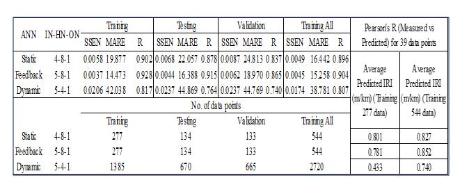
The numbers of the inputs, hidden nodes, and output layers are denoted by IN-HN-OH, respectively. All ANN types have IRI₀, cumulative ESAL, SN, and age as the independent variables. The feedback and dynamic AAN models consider the predicted IRI values from the static ANN as the additional independent variable. The models are verified using the same data sets used to verify the enhanced dummy regression equation. Based on the information given in Figure 07, the feedback ANN is the best network to be used for future IRI predictions. The sum of squared error of prediction (SSEN) and the mean absolute relative error (MARE) for the feedback ANN model are the lowest compared with other ANN models. The R values (measured vs. predicted) are the highest compared to other ANN models. The static ANN showed fairly good predictions. However, the data sets used for model verification do not fit the dynamic ANN analysis approach. Further analysis was conducted to compare the IRI values predictions using 277 and 544 training data sets. The results showed that the prediction using training all 544 data sets indicated higher R values for all three ANN types. The ANN models were compared, and the key findings are summarized;

• The R of 0.852 was observed for feedback ANN compared to 0.807 and 0.740 for static and dynamic ANNs, respectively. The observed percent difference is 37.9% for feedback ANN, 39.7% and 46% for the static and dynamic ANNs, respectively.
• Comparisons between the mean measured and predicted IRI values show that the enhanced dummy regression equation gave better prediction with only -2.9% differences compared to the feedback ANN model minimum errors of 37.9%.

Therefore, for similar kind of data sets, it is recommended to use feedback ANN with training all data sets to predict future IRI values.

Comparison between other IRI model with the Western region enhanced dummy regression equation

Table 02 summarizes the R values and percent differences of the measured vs. predicted data sets for test sections in California and Wyoming. Meegoda and Gao (2014) equation in the literature review section was verified and compared with the enhanced dummy regression equation developed for the LTPP Western region in this study.

Data sets from the test sections in California and Wyoming were used to represent no-freeze and freeze climate zones, respectively (FHWA, 2006). The observed R values are 0.724 and 0.456 for Equations 1 and 3, respectively. However, the enhanced dummy regression equation developed in this study showed a better prediction with only 17.6% difference between the measured and predicted mean IRI values compared to the model developed by Meegoda and Gao (2014). Further analysis on the data sets from the test sections in Wyoming showed that the R values between 0.2 to 0.5. The enhanced dummy regression equation’s prediction is better with 25% difference compared with the prediction using Equation 1, approximately 213% difference from the mean measured IRI value. Equation 1 showed poor predictions since three out of six test sections verified (56-2015, 56-2017, 56-2020) recorded percent differences more than 300% each. The equation developed in this study provides a consistent prediction compared to other equation. Therefore, it is feasible to use the enhanced dummy regression equation for future IRI prediction.

References

AASHO. (1962). The AASHO Road Test, Report 5, Pavement Research, Highway Research Board Special Report 61E. Washington, D.C.: National Research Council.
AASHTO. (1993). AASHTO design guide for guide for pavement structures. American Association of the State Highway and Transportation Officials, Washington, DC.
Attoh-Okine, N. O. (1994). Predicting roughness progression in flexible pavements using Artificial Neural Networks. In Transportation Research Board Conference Proceedings, 1(1), 55-62.
Federal Highway Administration (FHWA). (2006). Long-term pavement performance (LTPP) data analysis support: National pooled fund study TPF-5 (013). Effect of multiple freeze cycles and deep frost penetration on pavement performance and cost.
Federal Highway Administration (FHWA). (2009). Guidelines for implementing NCHRP1-37A M-E Design procedures in Ohio: Volume 4 – MEPDG models validation and recalibration. Washington, DC.: U.S Department of Transportation.
Kargah-Ostadi, N., Stoffels, S., & Tabatabaee, N. (2010). Network-level pavement roughness prediction model for rehabilitation recommendations. Transportation Research Record: Journal of the Transportation Research Board, 2155(1), 124-133.
Madanat, S., Nakat, Z., Farshidi, F., Sathaye, N., & Harvey, J. (2005). Development of empirical-mechanistic pavement performance models using data from the Washington State PMS database. Research Rep.
Meegoda, J., & Gao, S. (2014). Roughness progression model for asphalt pavements using Long Term Pavement Performance data. Journal of Transportation Engineering, 140 (8).
Mississippi Department of Transportation (MDOT). (2013). Implementation of MEPDG in Mississippi-Draft Final Mississippi DOT Pavement M-E Design User Guide. Report FHWA/MS-DOT-RD-013-170 MDOT. Mississippi : Jackson.
Mohamed Jaafar, Z. F., Ahlan, M., & Uddin, W. (2015). Modeling of pavement roughness performance using the LTPP database for southern region in the U.S. In 6th International Conference Bituminous Mixtures and Pavements, Thessaloniki.
Najjar, Y. M. (1990). Quick manual for TR-SEQ1. Developed at Department of Civil Engineering. Manhattan, Kansas, USA. : Kansas State University.
Uddin, W., Hudson, W. R., & Haas, R. (2013). Public Infrastructure Asset Management. McGraw-Hill, Inc.
Yasarer, H. I. (2013). Decision making in engineering prediction systems. (PhD Thesis). Kansas State University. Manhattan, Kansas.
Copyright information
This work is licensed under a Creative Commons Attribution-NonCommercial-NoDerivatives 4.0 International License.
About this article
Publication Date
26 December 2017
Article Doi
eBook ISBN
978-1-80296-950-4
Publisher
Future Academy
Volume
2
Print ISBN (optional)
-
Edition Number
1st Edition
Pages
1-882
Subjects
Technology, smart cities, digital construction, industrial revolution 4.0, wellbeing & social resilience, economic resilience, environmental resilience
Cite this article as:
Jaafar*, Z. F. M., Uddin, W., & Najjar, Y. M. (2017). Pavement Roughness Modeling Using Regression And Ann Methods For Ltpp Western Region. In P. A. J. Wahid, P. I. D. A. Aziz Abdul Samad, P. D. S. Sheikh Ahmad, & A. P. D. P. Pujinda (Eds.), Carving The Future Built Environment: Environmental, Economic And Social Resilience, vol 2. European Proceedings of Multidisciplinary Sciences (pp. 536-548). Future Academy. https://doi.org/10.15405/epms.2019.12.53