Gradient Neural Dynamics Based on Modified Error Function

Abstract

The present study is devoted to methods for the numerical solution to the system of equations=. In the case certain conditions are met, the classical gradient neural network (GNN) dynamics obtains fast convergence. However, if those conditions are not satisfied, solution to the equation does not exist and therefore the error function():=(t)- cannot be equal to zero, which increases the CPU time required for the calculation. In this paper, the solution to the matrix equation = is studied using the novel Gradient Neural Network (GGNN) model, termed as GGNN(,,). The GGNN model is developed using a gradient of the error matrix used in the development of the GNN model. The proposed method uses a novel objective function that is guaranteed to converge to zero, thus reducing the execution time of the Simulink implementation. The GGNN-based dynamical systems for computing generalized inverses are also discussed. The conducted computational experiments have shown the applicability and advantage of the developed method.

Keywords: Gradient neural network, generalized inverses, moore-penrose inverse, linear matrix equations

Introduction

In this study work, we deal with the real-time solutions of the general linear matrix equation (GLME) $AXB=D$ utilizing the gradient-established neural network (GNN) dynamical evolution, termed as GNN(,,). Previously, GNN models were described and investigated in the works of Wang (1992, 1993), Zhang et al. (2009), Wang (1997), Wei (2000), Wang and Li (1994), Ding and Chen (2005), Zhang and Chen (2008). Convergence investigation indicates that the output of GNN(,,) is specified by the choice of the initial state and belongs to the set of theoretical solutions to. Also, this work contains diverse applications of the GNN(,,) design described in Stanimirović et al. (2017, 2019, 2022) and improvements of proposed models for solving linear systems=described in Urquhart (1968). Most applications examined the impact of activation functions on the convergence rate of GNN(,,) theoretically and by means of simulation experiments. In the last section, we will test the novel gradient-based GNN formula (GGNN), which includes a different error matrix than the GNN model.

The implementation is defined on the set of real matrices and is based on making simulations of considered GNN-based models for solving matrix equations. The numerical experiments are tested in MATLAB Simulink.

Problem Statement

Recurrent neural networks (RNNs) form an essential class of methods for solving the matrix equations. RNNs are splitted into two categories: Gradient Neural Networks (GNN) and Zhang (or Zeroing) Neural Networks (ZNN). The GNN flow is explicit and efficient in solving time-invariant problems, which assumes constant coefficients matrices in underlying matrix equations. ZNN models are mostly implicit and efficient in solving time-varying problems (entries involved in coefficient matrices of the equations are functions of time $t\in \mathrm{R},\mathrm{}t>\mathrm{0}$).

General GNN neural dynamics are used to solve $AXB=D$. The dynamical evolution is developed based on the residual $E\left(t\right):=AV\left(t\right)B-D$, such that() is an unknown state-variable matrix which converges to the required matrix of the GLME $AXB=D$. The goal function $\mathrm{\epsilon }\left(t\right)={\left|\left|D-AV\left(t\right)B\right|\right|}_F^2/2$, is the function of the Frobenius norm. The gradient matrix of the objective $\mathrm{\epsilon }\left(t\right)$is computed as

$\frac{\partial \mathrm{\epsilon }\left(\mathrm{V}\left(\mathrm{t}\right)\right)}{\partial \mathrm{V}}=\frac{\mathrm{1}}{\mathrm{2}}\frac{\partial {\left|\left|D-AV\left(t\right)B\right|\right|}_{\mathrm{F}}^{\mathrm{2}}}{\partial \mathrm{V}}=-{\mathrm{A}}^{\mathrm{T}}\left(D-AV\left(t\right)B\right)B^{\mathrm{T}}$.

By the GNN evolution, one derives the dynamics

$\stackrel{\dot{}}{V}\left(t\right)=\frac{dV\left(t\right)}{dt}=-\mathrm{\gamma }\left(\frac{\partial \mathrm{\epsilon }\left(V\left(t\right)\right)}{\partial V}\right)=-\mathrm{\gamma }{A}^{\mathrm{T}}\left(AV\left(t\right)B-D\right)B^{\mathrm{T}}$,(1)

in which $\stackrel{\dot{}}{V}\left(t\right)$ is the time derivative and $\mathrm{}\mathrm{\gamma }>\mathrm{}\mathrm{0}$ is a positive gain parameter necessary for accelerating convergence. A faster convergence is achieved by increasing the value γ. We denote this model as GNN(,,). As already mentioned, the considered matrix-valued residual which cancels out over time is $E\left(\mathrm{t}\right)=D-AV\left(t\right)B$, such that() is the activation state variables matrix. The nonlinear GNN(,,) design is defined by

$\frac{\text{d}V\left(t\right)}{\text{d}t}=\stackrel{\dot{}}{V}\left(t\right)=\mathrm{\gamma }{A}^{\mathrm{T}}\mathcal{F}\left(D-AV\left(t\right)B\right)B^{\mathrm{T}}$.

The function array $\mathcal{F}\left(\mathrm{C}\right)$ includes any odd and monotonically-increasing activation function, which is applicable to each individual entry of its own matrix arguments.

The error function $E_G\left(t\right)$ is introduced using analogy with gradient-descent iterations for unconstrained nonlinear optimization. The residual $E\left(t\right)=AV\left(t\right)B-D$ is forced to the null matrix Stanimirović et al. (2018). The gradient of

${\mathrm{\epsilon }}_V=\frac{\left|\right|E\left(t\right){\left|\right|}_F^{\mathrm{2}}}{\mathrm{2}}=\frac{\left|\right|AV\left(t\right)B-D{\left|\right|}_F^{\mathrm{2}}}{\mathrm{2}}$

is equal to

$\frac{\partial {\epsilon }_V}{\partial V}=\nabla {\epsilon }_V=A^{\mathrm{T}}\left(AV\left(t\right)B-D\right)B^{\mathrm{T}}$.

The GNN dynamic evolution minimizes $\left|\right|AV\left(t\right)B-D{\left|\right|}_{\mathrm{F}}^{\mathrm{2}}$ and it is established on the direct correlation (1) among $\stackrel{\dot{}}{V}\left(t\right)$ and $\nabla {\epsilon }_V$ (Wang, 1993; Zhang et al., 2009; Wang, 1997).

Research Questions

The subsequent motivation questions were posed during the study:

• How to increase the speed of obtaining numerical solution of AXB=D?
• How to define the GNN design for solving AVtB=D established on the residual matrix EGt≔∇εVt=ATAVtB-DBT=ATEtBT?
• What is the convergence speed of the new dynamics which is developed on the basis of EGt?
• What is the numerical behaviour of the new model?

Purpose of the Study

The intention of this research is to find new GNN-type dynamical system based on a novel error functions.

Standard GNN design solves the GLME $AXB-D=0$under the condition $A{A}^{†}D{B}^{†}B=D$ (Stanimirović & Petković, 2018). Our aim is to avoid this constraint and originate dynamical evolutions based on the error function that tends to zero without restrictions.

Our motivation in defining new error function arises from gradient-descent methods for minimizing nonlinear multivariate functions. Our leading idea is the fact that the GLME $\nabla {\epsilon }_V=A^{\mathrm{T}}\left(AV\left(t\right)B-D\right)B^{\mathrm{T}}=0$ is convergent without restrictions. Results about solvability of GLME and general solutions are described in Wang et al. (2018).

Research Methods

To improve the standard GNN design, we introduced a new GGNN dynamical flow. More precisely, instead of using the classical error matrix $E\left(t\right)=D-AV\left(t\right)B$, we took for error matrix the right hand side of GNN model (1), i.e., the gradient of $\mathrm{\epsilon }$ of the GNN formula. That leads us to a new evolution

$E_G\left(t\right)=\frac{\mathrm{1}}{\mathrm{2}}\frac{\partial \mathrm{\epsilon }\left(V\left(t\right)\right)}{\partial V}=\frac{\mathrm{1}}{\mathrm{2}}\frac{\partial {\left|\left|D-AV\left(t\right)B\right|\right|}_F^{\mathrm{2}}}{\partial V}=-A^{\mathrm{T}}\left(D-AV\left(t\right)B\right)B^{\mathrm{T}}$.

We denote new error matrix with $E_G$, because the error function would take the value of the gradient and seek minimization over the gradient.

Next step is to define new model with this error matrix, calledGNN, or shortly GGNN. Let us define goal function ${\mathrm{\epsilon }}_G={\left|\left|E_G\right|\right|}_F^2$, whose gradient is equal to

$\frac{\partial {\mathrm{\epsilon }}_G\left(V\left(t\right)\right)}{\partial V}=\frac{{\partial ‖{\mathrm{A}}^{\mathrm{T}}\left(D-AV\left(t\right)B\right)B^{\mathrm{T}}‖}_F^{\mathrm{2}}}{\partial V}=-\mathrm{2}{A}^{\mathrm{T}}A\left(A^{\mathrm{T}}\left(D-AV\left(t\right)B\right)B^{\mathrm{T}}\right)B{B}^{\mathrm{T}}$.

Using the GNN-type evolution design, the dynamical system for GGNN formula is expanded as

$\stackrel{\dot{}}{V_G}\left(t\right)=\frac{\text{d}{V}_G\left(t\right)}{\text{d}t}=\mathrm{\gamma }{A}^{\mathrm{T}}A\left(A^{\mathrm{T}}\left(D-AV\left(t\right)B\right)B^{\mathrm{T}}\right)B{B}^{\mathrm{T}}$,

where $\mathrm{\gamma }>\mathrm{}\mathrm{0}$ scales the convergence. For a faster convergence, it is better to use greater values of γ, as in the GNN model. Hence, the corresponding nonlinear GGNN model is given by the following dynamics:

$\stackrel{\dot{}}{V}\left(t\right)=\mathrm{\gamma }{A}^{\mathrm{T}}A\mathcal{F}\left(A^T\left(D-AV\left(t\right)B\right)B^{\mathrm{T}}\right)B{B}^{\mathrm{T}}$, (2)

where $\mathcal{F}\left(\right)$ is an odd and monotonically increasing function array based on arbitrary monotonically increasing odd activation function $f\left(\cdot \right)$.

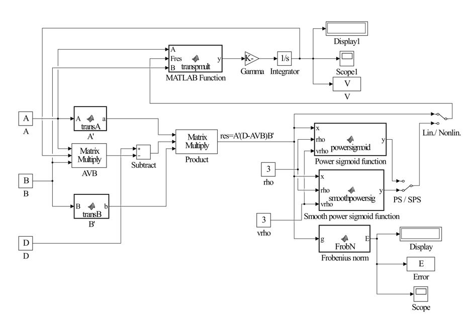
Figure 1 represents the Simulink implementation of GGNN(A,B,D) dynamics (2).

See Full Size >

Findings

In this section we perform numerical examples to examine the efficiency of the proposed GGNN model shown in Figure 1.

The subsequent activation functions $f\left(\cdot \right)$ are used in numerical experiments:

Linear activation function $f_{lin}\left(x\right)=x$

The Power-sigmoid activation function

$f_{ps}\left(x,\mathrm{}\rho ,\mathrm{}\varrho \right)=\left\{\begin{array}{c}{x}^{\rho },\mathrm{}\mathrm{}\mathrm{}\mathrm{}\mathrm{}\mathrm{}\mathrm{}\mathrm{}\mathrm{}\mathrm{}\mathrm{}\mathrm{}\mathrm{}\mathrm{}\mathrm{}\mathrm{}\mathrm{}\mathrm{}\mathrm{}\mathrm{}\mathrm{}\mathrm{}\mathrm{}\mathrm{}\mathrm{}\mathrm{}\mathrm{}\mathrm{}\mathrm{}\mathrm{}\mathrm{}\mathrm{}\mathrm{}\mathrm{}\mathrm{}\mathrm{}\mathrm{}\mathrm{}\left|x\right|\ge \mathrm{1}\\ \frac{\mathrm{1}+e^{-\varrho }}{\mathrm{1}-e^{-\varrho }}\bullet \frac{\mathrm{1}+e^{-\varrho x}}{\mathrm{1}-e^{-\varrho x}},\mathrm{}\mathrm{}\left|x\right|<\mathrm{1}\end{array}\right.$

The Smooth power-sigmoid activation function

$f_{sps}\left(x,\mathrm{}\rho ,\mathrm{}\varrho \right)=\frac{\mathrm{1}}{\mathrm{2}}{x}^{\rho }+\frac{\mathrm{1}+e^{-\varrho }}{\mathrm{1}-e^{-\varrho }}\bullet \frac{\mathrm{1}+e^{-\varrho x}}{\mathrm{1}-e^{-\varrho x}}$

In power-sigmoid activation function and smooth power-sigmoid activation function $\mathrm{\varrho }>\mathrm{2},\mathrm{}\mathrm{\rho }\ge \mathrm{3}$ is odd integer. We will assume $\varrho =\mathrm{}\rho =\mathrm{3}$ for all examples.

The Matlab command “ = rand()*rand()” is used to generate a random× matrix of rank.

Table 1 shows experimental results for square regular and non-regular random matrices of dimensions×. Table 2 shows experimental results obtained on regular and singular matrices of dimensions×. Here, NRT means that no result was obtained in a reasonable time. Experiments were conducted on computer with processor Intel(R) Core(TM) i5-10210U CPU @ 1.60GHz 2.11 GHz, 8 GB of RAM and Windows 10 OS. MatLab Version: R2021a.

Figure 2 illustrate trajectories of residual errors $\left|\left|D-AV\left(t\right)B\right|\right|$ for different activation functions. The graphs included in this figure show faster convergence of nonlinear GGNN models with respect to the linear GGNN.

See Full Size >

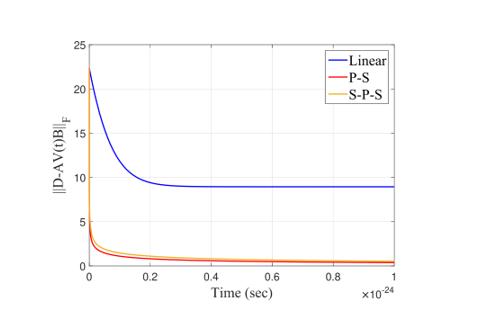
Figure 3 demonstrates a comparison of convergence rates of GNN and GGNN.

See Full Size >

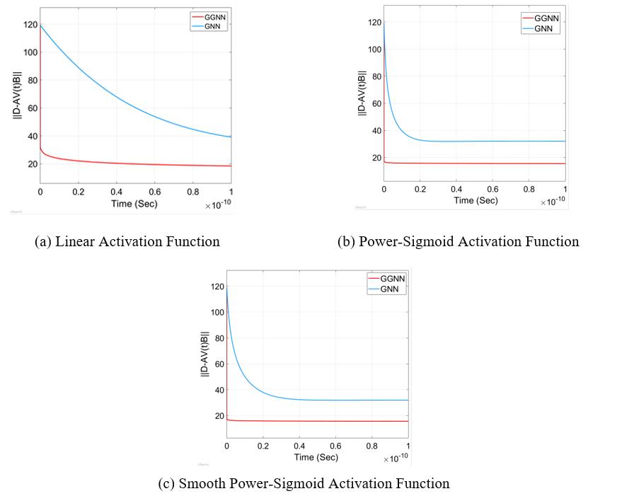
Figure 3 clearly shows a faster convergence of the GGNN model again the GNN dynamics.

Conclusion

In this paper, we proposed a new method for solving the equation $AXB=D$ using the replacement of the error function and introducing a new recurrent model of GGNN. The experimental results showed that the proposed model GGNN faster converges than the GNN model without losing quality for various dimensions and ranks. Further, a non-linear activation function speeds up the convergence compared to the linear activation function for all studied cases.

Other important achievement is the fact that proposed GGNN solved all tested equations even when GNN was not able to finish computations in reasonable time.

Acknowledgments

Predrag Stanimirović is supported by the Science Fund of the Republic of Serbia, (No. 7750185, Quantitative Automata Models: Fundamental Problems and Applications - QUAM). This work was supported by the Ministry of Science and Higher Education of the Russian Federation (Grant No. 075-15-2022-1121).

References

• Ding, F., & Chen, T. (2005). Gradient based iterative algorithms for solving a class of matrix equations. IEEE Transactions on Automatic Control, 50(8), 1216-1221. DOI:

  Google Scholar

  Crossref

• Stanimirović, P. S., Ćirić, M., Stojanović, I., & Gerontitis, D. (2017). Conditions for Existence, Representations, and Computation of Matrix Generalized Inverses. Complexity, 1-27. DOI:

  Google Scholar

  Crossref

• Stanimirović, P. S., & Petković, M. D. (2018). Gradient neural dynamics for solving matrix equations and their applications. Neurocomputing, 306, 200-212. DOI:

  Google Scholar

  Crossref

• Stanimirović, P. S., Petković, M. D., & Gerontitis, D. (2018). Gradient neural network with nonlinear activation for computing inner inverses and the Drazin inverse. Neural Processing Letters, 48(1), 109-133. DOI:

  Google Scholar

  Crossref

• Stanimirović, P. S., Petković, M. D., & Mosić, D. (2022). Exact solutions and convergence of gradient based dynamical systems for computing outer inverses. Applied Mathematics and Computation, 412, 126588. DOI:

  Google Scholar

  Crossref

• Stanimirović, P. S., Wei, Y., Kolundžija, D., Sendra, J. R., & Sendra, J. (2019). An application of computer algebra and dynamical systems. Proceedings of International Conference on Algebraic Informatics, 225-236. DOI:

  Google Scholar

  Crossref

• Urquhart, N. S. (1968). Computation of generalized inverse matrices which satisfy specified conditions. SIAM Review, 10(2), 216-218. DOI:

  Google Scholar

  Crossref

• Wang, G., Wei, Y., & Qiao, S. (2018). Generalized Inverses: Theory and Computations, Developments in Mathematics 53. Springer. Science Press. DOI:

  Google Scholar

  Crossref

• Wang, J. (1992). Electronic realisation of recurrent neural network for solving simultaneous linear equations. Electronics Letters, 28, 493-495. DOI:

  Google Scholar

  Crossref

• Wang, J. (1993). A recurrent neural network for real-time matrix inversion. Applied Mathematics and Computation, 55(1), 89-100. DOI:

  Google Scholar

  Crossref

• Wang, J. (1997). Recurrent neural networks for computing pseudoinverses of rank-deficient matrices. SIAM Journal on Scientific Computing, 18(5), 1479-1493. DOI:

  Google Scholar

  Crossref

• Wang, J., & Li, H. (1994). Solving simultaneous linear equations using recurrent neural networks. Information Sciences, 76(3-4), 255-277. DOI:

  Google Scholar

  Crossref

• Wei, Y. (2000). Recurrent neural networks for computing weighted Moore–Penrose inverse. Applied Mathematics and Computation, 116(3), 279-287. DOI:

  Google Scholar

  Crossref

• Zhang, Y., & Chen, K. (2008). Comparison on Zhang neural network and gradient neural network for time-varying linear matrix equation AXB=C solving. Proceedings of 2008 IEEE International Conference on Industrial Technology, 1-6. DOI:

  Google Scholar

  Crossref

• Zhang, Y., Chen, K., & Tan, H. Z. (2009). Performance analysis of gradient neural network exploited for online time-varying matrix inversion. IEEE Transactions on Automatic Control, 54(8), 1940-1945. DOI:

  Google Scholar

  Crossref