Matrix Data Processing Technology For Resource Saving

Abstract

The problem of resource saving on the example of geometric location of objects is considered. Such processes are known as problems of cutting, packing and geometrical covering. The majority of these problems are NP-hard. Nowadays there are still no algorithms of polynomial complexity to find optimum solutions for the above problems. Therefore, in the modern world much attention is paid to the study and development of approximate efficient algorithms for their solution. In practice, it is profitable to use heuristic multi-pass algorithms. They make it possible to find a rational solution but do not guarantee the optimum. The paper describes the matrix data processing technology to construct solutions for geometrical location problems. Thus, it is possible to form different variants of algorithms with a common structure. And further study of the effectiveness of the obtained algorithms allows us to determine the best of them. This process is described in the given paper. The estimation of efficiency of algorithms constructed on the basis of the described technology is checked on the example of the solution of a two-criterion complex problem of geometrical location. The stages of solving the problem are described. The computing experiment results based on the specially generated non-waste examples with a unitary coefficient of covering and cutting are given. The variants of the algorithm for the rational use of resources are determined.

Keywords: Problem of geometrical coveringresource saving

Introduction

Technological processes often use the step of item cutting or location taking into account their geometric peculiarities. This step is urgent for resource saving and it is difficult for decision making.

Currently, many scientists are developing effective algorithms for practical problems of resource saving ( Bouaine, Lebbar, & Ha, 2018; Kallrath, Rebennack, Kallrath & Kusche, 2014; Kartak, Marchenko, Petunin, Sesekin, & Fabarisova, 2017; Kartak & Ripatti, 2018; Kulga & Menshikov, 2014; Lua & Huang, 2015; Paquay, Schyns, & Limbourg, 2016; Rothe & Reyer, 2017).

Technological process is the way to design solutions and to create various algorithms with a common structure. The paper summarizes several techniques of developing and creating algorithms to solve geometrical location problems.

We can list basic problems of geometrical location ( Filippova & Valiakhmetova, 2014; Wang & Wascher, 2002):

• Linear (one-dimensional) material cutting;

• Cutting of sheets to rectangular items;

• Packing three-dimensional containers;

• Cutting and location of shaped objects in the given area;

• Maximum covering of linear material;

• Rectangular geometrical covering.

The classification of basic models for geometrical location problems is given in ( Dykhoff, 1990; Mukhacheva, Mukhacheva, Valeeva, & Kartak, 2004).

The problem of optimum geometrical location occurs in practice both as an autonomous problem and as a sub-problem. Besides, complex problems are being researched nowadays. The first example is a problem of geometrical covering and cutting ( Filippova & Valiakhmetova, 2014), where it is required to find a plan of covering some area (for example, floor) and a plan of cutting some material to covering items (for example, linoleum). The problem is a double-criterion one: it is needed to minimize the material consumption and to maximize the covering items’ sizes. Another variant of developing a combined cutting-covering problem represents a problem of covering some special technical objects, such as shells, with sheet material ( Kulga & Menshikov, 2014).

Despite a great variety of the location problems, all of them have the same structure. There exist two groups of objects, and a correspondence between the elements of these groups is established and estimated. This structure makes it possible to develop and use similar approaches to generating solutions for different problems.

Problem Statement

To begin, we examine a complex problem of geometrical covering and cutting . Some information concerning MOP (multi-coherent orthogonal polygon) and rectangular resource sizes are given and it is required to find the MOP covering plan and the plan of rectangular resource cutting to covering elements, at that it is necessary to maximize the covering elements’ sizes and to minimize the consumption (area or amount) of the resource to be cut. This problem is formalized by a mathematical model of the problem with two goal functions.

To describe MOP covering areas we enter the rectangular coordinate system: here the axes Ox and Oy coincide correspondingly with the bottom and the left flanks of the rectangle that goes round the covering area (Figure 01 ,a). Wand L denote the width and the length of the rectangle enveloping MOP. Location of each rectangular prohibited zone Bν is defined by coordinates ( χ _ν , η _ν ) of its bottom left corner and by sizes ${\omega }_{\nu },{\lambda }_{\nu },\nu =\stackrel{-}{1,\mu }$, where μ is the number of prohibited zones.

See Full Size >

Research Questions

Given : MOP to be covered is denoted by the set $P=〈W,L,({\chi }_{\nu },{\eta }_{\nu }),({\omega }_{\nu },{\lambda }_{\nu }),\nu =\stackrel{-}{1,\mu }〉$. Besides, there is a non-limited number of rectangular sheets of length Θ and width h (for problems with resource of sheets), or there is a semi-endless roll of width h, which is to be cut to rectangular items (Figure 01 , b). There is also some information about waste material in the form of a set of rectangular items K = ( k ₁, k ₂, … k _τ ) with sizes $l_j^{+}\times w_j^{+},j=\stackrel{-}{1,\tau }$.

Required: to find a plan of covering MOP P ; a plan of cutting of rectangular resource to rectangular items; to minimize the function values, characterizing the efficiency of solution for geometrical covering and cutting sub-problems:

$$\begin{array}{}\mathrm{m}\mathrm{i}\mathrm{n}{F}_{\mathrm{c}\mathrm{o}\mathrm{v}}\left(T\right)=\underset{i=1}{\overset{m}{\sum }}\left(l_i+w_i\right).\end{array}$$

$$\begin{array}{}\mathrm{m}\mathrm{i}\mathrm{n}{F}_{\text{cut}}\left(T\right)=\left\{\begin{array}{c}{N}^{РЛ},\text{\hspace{0.17em}for rectangular sheets;}\\ L^{РП}=\underset{i=\mathrm{1}..m}{\mathrm{m}\mathrm{a}\mathrm{x}}\left({x^{\text{'}}}_i+l_i\right)\text{,\hspace{0.17em}for semi-endless strip}\end{array}\right.\end{array}$$

Where $T=\left\{m,w=(w_1,w_2,...,w_m),l=(l_1,l_2,...,l_m)\right\}$

is a set of m rectangular items with the sizes $w_i\times l_i,i=\stackrel{-}{1,m}$, they cover MOP and are subjected to be cut out of the resource and wastes; l _i , w _i are the length and width of the covering item $t_i\in T$, $T=Q\cup K^{+}$, where Q is a number of rectangular items covering MOP, the items are cut out of the standard resource; K ⁺ is a set of rectangular items that are cut out of the waste material; N ^sheet is a number of the used rectangular sheets (in case the cutting problem uses the sheet resource); L ^strip is the length of the occupied part of a semi-endless strip (in case the cutting problem uses the roll resource), $L^{strip}=\underset{i=\mathrm{1}..m}{\mathrm{m}\mathrm{a}\mathrm{x}}\left({x^{\text{'}}}_i+l_i\right);{x^{\text{'}}}_i,{y^{\text{'}}}_i$ are coordinates of the left bottom angle of a rectangle with the number i in the plan of rectangular resource cutting (in the frame of axes of rectangular resource).

To formalize the problem, we enter some additional variables $z_{ij}^x$, $z_{ij}^y$, ${\tilde{z}}_{i\nu }^x$ and ${\tilde{z}}_{i\nu }^y$, so that $z_{ij}^x=1$ ( $z_{ij}^y=1$), if the rectangular element’s projection I on the axis Ох ( Оу ) is lower than the projection of the rectangular element j on the axis Ох ( Оу ), otherwise $z_{ij}^x=0$ ( $z_{ij}^y=0$); ${\tilde{z}}_{i\nu }^x=1$ ( ${\tilde{z}}_{i\nu }^y=1$), if the rectangular item projection i on the axes Ох ( Оу ) is to the left (lower) of the prohibited zone projection v on the axis Ох ( Оу ), otherwise ${\tilde{z}}_{i\nu }^x=0$ ( ${\tilde{z}}_{i\nu }^y=0$).

Then it is necessary to find the following:

1. A set T of rectangular items covering MOP P and the corresponding covering plan, that is, for every $t_i\in T$ it is needed to find a set of values $〈x_i,y_i,l_i,w_i〉$, where x _i , y _i are coordinates of the item’s left bottom corner in the coordinate system of the area P ; l _i , and w _i are the length and the width of a rectangular item correspondingly, so that:

$$\begin{array}{}\text{(1)}& l_i\le h,w_i\le \mathrm{\Theta },i=\stackrel{-}{1,m},\left(1\right)\end{array}$$

$$\begin{array}{}\text{(2)}& x_i+l_i\le L,y_i+w_i\le W,i=\stackrel{-}{1,m},\left(2\right)\end{array}$$

$$\begin{array}{}\text{(3)}& x_i\ge 0,y_i\ge 0,i=\stackrel{-}{1,m},\left(3\right)\end{array}$$

$$\begin{array}{}\text{(4)}& z_{ij}^x+z_{ji}^x+z_{ij}^y+z_{ji}^y\ge 1,i=\stackrel{-}{1,m},j=\stackrel{-}{1,m},i\ne j\left(4\right)\end{array}$$

$$\begin{array}{}\text{(5)}& y_j\ge y_i+w_i-W\left(1-z_{ij}^y\right),i=\stackrel{-}{1,m},j=\stackrel{-}{1,m},\left(5\right)\end{array}$$

$$\begin{array}{}\text{(6)}& x_j\ge x_i+l_i-L\left(1-z_{ij}^x\right),i=\stackrel{-}{1,m},j=\stackrel{-}{1,m},\left(6\right)\end{array}$$

$$\begin{array}{}\text{(7)}& {\tilde{z}}_{i\nu }^x+{\tilde{z}}_{\nu i}^x+{\tilde{z}}_{i\nu }^y+{\tilde{z}}_{\nu i}^y\ge 1,i=\stackrel{-}{1,m},\nu =\stackrel{-}{1,\mu },\left(7\right)\end{array}$$

$$\begin{array}{}\text{(8)}& {\eta }_{\nu }\ge y_i+w_i-W\left(1-{\tilde{z}}_{i\nu }^y\right),i=\stackrel{-}{1,m},\nu =\stackrel{-}{1,\mu },\left(8\right)\end{array}$$

$$\begin{array}{}\text{(9)}& {\chi }_{\nu }\ge x_i+l_i-L\left(1-{\tilde{z}}_{i\nu }^x\right),i=\stackrel{-}{1,m},\nu =\stackrel{-}{1,\mu },\left(9\right)\end{array}$$

$$\begin{array}{}\text{(10)}& \underset{i=1}{\overset{m}{\sum }}{w}_i\cdot l_i=S_{MOP}\left(10\right)\end{array}$$

The conditions ( 1 ) impose restrictions on the sizes of covering rectangular item: they must not exceed the size of the rectangular resource. The conditions ( 2 ) and ( 3 ) specify the admissible position of rectangular items in the MOP: they must not exceed the boundaries of the MOP. The conditions ( 4 ) – ( 6 ) provide non-overlapping of rectangular items with each other; the conditions ( 7 ) – ( 9 ) provide non-overlapping of rectangular items with prohibited zones. The condition ( 10 ) describes necessity of full geometrical covering of the MOP with rectangular items without gaps.

2. The plan to cut the orthogonal resource to rectangular items of the set T is such as to meet the following conditions:

$$\begin{array}{}\text{(11)}& x_i^{\text{'}}\ge 0,y_i^{\text{'}}\ge 0,i=\stackrel{-}{1,m},\left(11\right)\end{array}$$

$$\begin{array}{}\text{(12)}& x_i^{\text{'}}+l_i\le \Theta ,y_i^{\text{'}}+w_i\le h,i=\stackrel{-}{1,m},\left(12\right)\end{array}$$

$$\begin{array}{}\text{(13)}& z_{ij}^x+z_{ji}^x+z_{ij}^y+z_{ji}^y\ge \mathrm{1},i=\stackrel{-}{\mathrm{1},m},j=\stackrel{-}{\mathrm{1},m},i\ne j,\mathrm{}\left(\mathrm{13}\right)\end{array}$$

$$\begin{array}{}\text{(14)}& y_j^{\mathrm{\text{'}}}\ge y_i^{\mathrm{\text{'}}}+w_i-W\left(\mathrm{1}-z_{ij}^y\right),i=\stackrel{-}{\mathrm{1},m},j=\stackrel{-}{\mathrm{1},m},\mathrm{}\left(\mathrm{14}\right)\end{array}$$

$$\begin{array}{}\text{(15)}& x_j^{\mathrm{\text{'}}}\ge x_i^{\mathrm{\text{'}}}+l_i-L\left(\mathrm{1}-z_{ij}^x\right),i=\stackrel{-}{\mathrm{1},m},j=\stackrel{-}{\mathrm{1},m},\mathrm{}\left(\mathrm{15}\right)\end{array}$$

The conditions ( 11 ) – ( 12 ) provide admissible location of rectangular items inside the orthogonal resource; the conditions ( 13 ) – ( 15 ) ensure that rectangular items do not overlap each other.

The goal functions min F _cov(T) and min F _cut(T) make it possible to compare the quality of different solutions for the same problem, but do not make it possible to compare the solution efficiency for different problems as their values depend on the initial data, for example, on the sizes of the resource and of the MOP.

That is why the quality of solutions is also estimated with the help of two relative indicators:

• For the geometrical covering problem we calculate the covering coefficient $k_{\mathrm{c}\mathrm{o}\mathrm{v}}=\frac{S_{MOP}}{P_T}·\frac{P_{\text{resourse}}}{S_{\text{resourse}}}$,

where S _MOP and S _resourse are the areas of the MOP and the resource correspondingly, P _T and P _resourse are summarized perimeters of the covering items and of the resource correspondingly;

• For the orthogonal cutting problem we define the cutting coefficient as follows $k_{cut}=\frac{\stackrel{m}{\underset{i=1}{\sum }}{w}_i·l_i}{S_{\text{resourse}}}$.

The geometrical covering coefficient equals 1, if joints of the covering items are only on the boundaries of MOP and do not go into the inner area, otherwise k _cov  < 1.

If the problem is solved without any waste material the cutting coefficient equals 1, otherwise k _cut  < 1.

The covering and cutting coefficients contradict each other because maximization of the sizes of covering items results in decrease of the cutting coefficient (waste increases). And vice versa, when the sizes of cutting elements are small, the cutting coefficient increases but the covering one decreases.

Purpose of the Study

The study of algorithms for solving cutting-packing problems has shown that there exist several common approaches, i.e. technologies, to developing and designing new algorithms. The paper ( Dyaminova & Filippova, 2016) describes the following technologies of designing algorithms for solving geometrical location problems: layer-by-layer; level; non-level; block; matrix; based on special geometric structures. The level and matrix technologies are used for designing algorithms to solve the formulated above problem.

Application of the level technology for the complex problem of geometrical covering and cutting is based on sequential execution of algorithms for solving each of the following stages (sub-problems).

Stage I: decomposition of MOP.

The geometrical component of the above problem makes imposes certain difficulties in the transformation of information while designing solutions. It is connected with geometrical peculiarities of the area in which items are located. This stage is aimed at describing the initial MOP as a set of rectangular areas to be covered.

To solve this stage, the authors of the given paper use a level algorithm ( Simonis & O’Sullivan, 2008) and a matrix method of presenting geometric information ( Dyaminova & Filippova, 2016).

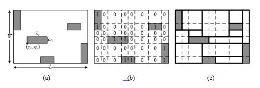
Every area to be covered is presented as a matrix in the above algorithm of ( Dyaminova & Filippova, 2016). In the 2D matrix every cell represents a pixel on a plane. The matrix elements show whether an area is uncovered, or once-covered or iteratively-covered by geometrical items.

Earlier, the authors of the given paper proposed an algorithm based on the matrix method to solve the following problem.

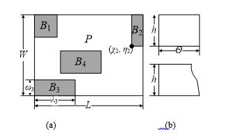
The rectangle location problem in a multi-coherent orthogonal polygon (MOP). There is given an orthogonal polygonal area, it is enveloped by a rectangle with the known width W and length L , and there are given the co-ordinates ( χ _ν , η _ν ) and the sizes ( ω _ν ,  λ _ν ), $\nu =\stackrel{-}{1,\mu }$

of rectangular obstacles inside the area (Figure 02 a). It is required to find the plan for location of rectangular item with the maximum coefficient of location.

The algorithm based on the matrix technology of designing rectangular item location inside a polygonal area is described in detail in ( Dyaminova & Filippova, 2016), where the MOP presents a two-dimensional binary array.

All faces of the obstacles are lined through. So the area with obstacles becomes covered with a network (Figure 02 b), each cell of which either does not contain any obstacle (value «0» in the binary matrix), or represents an obstacle or a part of it (value «1» in the binary matrix). Then an initial empty cell is chosen (for example, left bottom one), and according to some criterion the adjacent empty cells are integrated into a rectangular box starting with the first chosen. Possible criteria to choose the direction of integration are as follows: horizontal, vertical, diagonal (alternation of horizontal and vertical), random choice of direction (equiprobable; user-defined – when manually done; proportional - when the choice depends on the area’s length and width). The integration continues till the moment when an obstacle is encountered, after that a new initial cell is found and all steps are repeated. The process goes on until all empty cells are referred to some rectangular area (box). As a result, the original MOP is divided into rectangular domains into which rectangular items are to be located (Figure 02 c). Thus, the problem goes down to the 2D packing problem.

The algorithms based on matrix technology have shown high efficiency on both real and generated test examples of problems of rectangular location and of geometrical covering ( Dyaminova & Filippova, 2016; Kulga & Menshikov, 2014).

See Full Size >

Stage II: geometrical covering.

The covering plan to each area is found provided that rectangular items to be located are of the maximum size for the given resource. It means that the sub-problem of geometrical covering for the rectangular area is being solved. For this, the following can be used:

• the simple single-pass algorithm “bottom left” ( Chazelle, 1983), it starts working from the uncovered bottom left point and covers the area with a rectangle of the maximum admissible size at every pace;

• the algorithm offered in, it is a modification of the sequential value correction ( Mukhacheva et al., 2004) and it takes into account the covering resource excess expenditure; it is a multi-pass algorithm that makes it possible to find the local-optimum covering plan;

• the multi-pass algorithm of local search for optimum based on the evolutional strategy ( Mukhacheva et al., 2004).

Stage III: orthogonal cutting.

At the last stage, a cutting sub-problem is solved, when it is required to find the plan for cutting resource to covering items. Any known algorithm for solving the rectangular packing problem can be used here. For this purpose we used the following:

• fast one-pass algorithm “first fitting”;

• multi-pass algorithm of sequential value correction ( Mukhacheva et al., 2004), it takes account of the per-detail expenses when the ordered sequence of items to be cut is generated;

layer-by-layer algorithm with values ( Dyaminova & Filippova, 2016), based on the layer-by-layer technology that takes account of the per-detail material consumption rate.

Research Methods

In the described below series of experiments, as test examples we used some specially generated initial data providing the so-called non-waste solution for the problem. In such examples there exist a solution (the covering plan and the cutting plan) when coefficients of geometrical covering and of cutting both equal 1.

Experiment №1; Comparison of effectiveness of the level method and the matrix one for designing the general algorithms of a complex problem of geometrical covering and cutting on non-waste examples.

These are the three-step methods of solving the problem, here at each step one sub-problem is solved by one of the possible algorithms. The output information of one sub-problem becomes the initial data for the next problem. We have investigated the efficiency of two general algorithms in which simple heuristics are used for solving sub-problems of covering and cutting. They are:

• one algorithm M1 based on the matrix technology that uses the following:

  • stage 1 – the sub-problem of MOP decomposition: matrix decomposition algorithm,

  • stage 2 – the geometrical covering sub-problem: - “bottom left” algorithm,

  • stage 3 – the cutting sub-problem: “first fitting” algorithm;

• another algorithm L1 based on the level technology that employs the following:

  • stage 1 – the problem of MOP decomposition: level algorithm,

  • stage 2 – the geometrical covering sub-problem: - “bottom left” algorithm,

  • stage 3 – the cutting sub-problem: “first fitting” algorithm.

Ten non-waste problems have been solved and the results of the experiment №1 are shown in the tables 01 and 02 .

As one can see from the tables 01 and 02 , when the algorithm based on the matrix technology is used, it results in higher efficiency of solution: the cutting coefficient differs insignificantly on average. However, the geometrical covering coefficient is a bit higher on average if the matrix algorithm is used.

So we have used the matrix algorithms in the next experiment for researching the effectiveness of the algorithm variants based on one technology.

Experiment №2. Research of the effectiveness of different algorithm combinations to solve the sub-problems that compose variants of the matrix algorithms for solving problems of geometrical covering and cutting

The effectiveness of nine general algorithms on the basis of the matrix technology has been studied. The following algorithms were used for solving sub-problems at each stage:

stage 1 – the sub-problem of MOP decomposition: matrix decomposition algorithm ( M ),

stage 2 – the geometrical covering sub-problem: “bottom left” algorithm ( BL ), sequential value correction algorithm ( V ); evolutional algorithm ( E );

stage 3 – the cutting sub-problem: “first fitting” algorithm ( F ), sequential value correction algorithm ( V ), layer-by-layer algorithm with values ( L ).

Thus, we received the following variants of the general algorithm M+BL+F (M1), M+BL+V (M2), M+BL+L (M3), M+V+F (M4), M+V+V (M5), M+V+L (M6), M+E+F (M7), M+E+V (M8), M+E+L (M9) .

Tables 03 and 04 show the results of each of the 10 non-waste problems generated at random and the average values of the geometrical covering coefficient and of the cutting one. The highlighted cells show the best variants in the column.

On average, the best result for solving a complex problem, from the point of view of geometrical covering efficiency, is received with the help of the combination M+E+L (M9), in case when the evolutional algorithm is used to solve the geometrical covering sub-problem and the layer-by-layer algorithm with values to solve the orthogonal cutting sub-problem. All other algorithm combinations are considerably behindhand as for the geometrical covering coefficient is concerned, both in separate examples and on average.

Findings

The algorithm combination M+E+V (M8) shows the best result for the orthogonal cutting sub-problems. At the stage of solving the geometrical covering sub-problem, the evolutional algorithm was used. At the stage of solving the orthogonal cutting sub-problem, the sequential value correction algorithm was applied. It is worth noting that other algorithm combinations also result in quite efficient solutions. The orthogonal cutting coefficient differs insignificantly in cases with M+V+L (M6) and M+V+F (M4) combinations. It occurs when the sequential value correction algorithm is used at the stage of solving the geometrical covering sub-problems, and the layer-by-layer with values algorithm and the first fitting one are applied at the stage of solving the orthogonal cutting sub-problem. It is also significant that only one algorithm variant shows the optimal solution for the cutting sub-problem. It is the algorithm with M+BL+L (M3) combination. Neither variant gives the optimal covering plan.

Conclusion

We propose schemes of implementation of variants of algorithms for solving the complex problem of geometrical covering and cutting, these variants are based on the level and the matrix technologies. One of the computing experiments has shown the advantage of the matrix technology as far as the covering quality is concerned. The structure of the matrix technology made it possible to realize nine variants of the matrix algorithm for solving the complex problem. The computing experiment singled out the best of them from the point of view of effectiveness of covering and cutting.

We have used the special non-waste examples with preset optimal plans of covering and cutting to evaluate the efficiency and we come to conclusion that neither algorithm under consideration has got the optimal solution. It means that it is necessary to keep on improving the ways of designing algorithms for solving NP-hard complex problems of geometrical covering and cutting.

Acknowledgments

The work is supported by Russian fund of fundamental research (project 19-07-00895, 19-07-00780).

References

1. Bouaine, A., Lebbar, M., & Ha, M. A. (2018). Minimization of the wood wastes for an industry of furnishing: a two dimensional cutting stock problem. Management and Production Engineering Review, 9(2), 42-51.
2. Chazelle, B. (1983). The bottom-left bin packing heuristic: An efficient implementation. IEEE Trans. on Comput, 2, 697-707.
3. Dyaminova, E. I., & Filippova, A. S. (2016). Technologies of decisions designing in problems of geometrical placing. Applied mathematics and fundamental informatics: annual scientific log, 3, 134-141.
4. Dykhoff, H. (1990). A typology of cutting and packing problems. European Journal of Operational research, 44, 145-159.
5. Filippova, A. S., & Valiakhmetova, J. I. (2014). Optimal use of resources: cutting-packing problems. Advances in economics and optimization: collected scientific studies dedicated to the memory of L. V. Kantorovich / editors, Leon A. Petrosyan, Joseph V. Romanovsky & David Wing-kay Yeung, 37-50.
6. Kallrath, J., Rebennack, S., Kallrath, J., & Kusche, R. (2014). Solving real-world cutting stock-problems in the paper industry: Mathematical approaches, experience and challenges. European Journal of Operational Research, 238, 374–389.
7. Kartak, V. M., Marchenko, A. A., Petunin, A. A., Sesekin, A. N., & Fabarisova, A. I. (2017). Optimal and heuristic algorithms of planning of low-rise residential buildings.  Electronic Materials, 14, 234-235.
8. Kartak, V. M., & Ripatti, A. V. (2018). The minimum raster set problem and its application to the d-dimensional orthogonal packing problem. European Journal of Operational Research, 271(1), 33-39.
9. Kulga, K. S., & Menshikov, P. V. (2014). Optimizatsiyia geometricheskogo pokrytiya mnogo kogerentnogo ortogonalnogo mnogougolnika s granichnymi prepyatstviyami s uchetom konstruktivnykh i tekhnologicheskikh ogranicheny [Optimization of geometrical covering of the multi-coherent orthogonal polygon with boundary obstacles taking into account design and technological restrictions]. Vestnik RGTRU, 4(50), part 2, 75-82.
10. Lua, H. C., & Huang, Y. H. (2015). An efficient genetic algorithm with a corner space algorithm for a cutting stock problem in the TFT-LCD industry. European Journal of Operational Research, 246, 51–66.
11. Mukhacheva, E. A., Mukhacheva, A. S., Valeeva, A. F., & Kartak, V. M. (2004). Methods of local search in tasks of orthogonal cutting and packing: review and prospects of development. Information Technologies, 5, annex, 2-17.
12. Paquay, C., Schyns, M., & Limbourg, S. (2016). A mixed integer programming formulation for the three-dimensional bin-packing problem deriving from an air cargo application. International Transactions in Operational Research, 23, 187–213.
13. Rothe, M., & Reyer, R. (2017). Process Optimization for Cutting Steel-Plates Proc. of the 6th International Conference on Operations Research and Enterprise Systems ICORES 2017, 27-37.
14. Simonis, H., & O’Sullivan, B. (2008). Search strategies for rectangle packing. LNCS, 5202, 52–66.
15. Wang, P., & Wascher, G. (2002). Special issue: Cutting Packing Problems. European Journal of Operational research, 141.