Student'S Distributions As An Alternative To Sustainable Distributions In The Digital Economy

Abstract

As the digital economy evolves, the data used for statistical analysis becomes more complex, dynamic, and the normal distribution law used to describe more trivial data becomes less suitable for describing complex processes. In this regard, the article is devoted to the study of the Student's distribution as an alternative to stable distribution laws, including the normal one. The article considers the main properties of stable distributions of statistics, their representation through the characteristic exponent, as well as the Student's distribution with n degrees of freedom. The interrelationships of these distribution classes are shown, as well as their differences. The paper also describes the meaning of Kolmogorov-Smirnov's consent criterion, which has been repeatedly applied in the practical part of the study. Using Python 3 programming language on the Jupyter Notebook platform, a statistical analysis of the XRP (Ripple) cryptocurrency course for 365 calendar days in 2018 was carried out. The analysis consists in testing three main hypotheses: H1, H2, H3 about subordination of the XRP course to the Student's distribution, the normal law of distribution and the Cauchy distribution, respectively. The analysis has shown that the studied data are indeed subject to the Student's distribution at the level of significance α less than 0.09043713341694139. Testing of H2, H3 hypotheses has shown that the normal law of distribution and distribution of Cauchy is not suitable for describing the rate of cryptocurrency for 2018 and the hypotheses were rejected.

Keywords: Student's distributionstable distributionnormal distribution lawKolmogorov-Smirnov testа

Introduction

The concept of "sustainable distribution" was first introduced by the French mathematician P. Levi in 1925. The concept was formulated as a result of studying the properties of the sum of independent equally distributed random variables. However, the practice of applying stable laws already existed in 1919 in astronomy. Later this type of distribution began to be introduced in other scientific spheres, such as economics, physics, chemistry, geology.

Sustainable distribution laws have also become widely applied in the financial sphere. Stochastic processes with stably distributed increments replaced the variants of Brownian motion based on normal distribution, with which the analysis of dynamics of financial indicators (prices and return on assets) in a continuous period of time was connected. Mandelbrot's first arguments against "normality" were made in 1963, showing empirically that asset price dynamics included a discrete component. He described the dynamics of the price increment process as a diffusion process like Levi with infinite dispersion ( Morozova & Pirlik, 2009).

Problem Statement

The problem with this issue is that from year to year, all statistical systems become more dynamic and it is impossible to use the normal distribution law for statistical analysis. With the advent of heavy tails, the Student's distribution begins to be used as an alternative to the Student's distribution, but the Student's distribution is rarely used for data analysis, especially for cryptocurrency. The distribution of the Student as a severe tailed one is not yet fully investigated, and this study will help to get an overview of this type of distribution.

Research Questions

Stable distributions and their properties. The law of distribution of a random variable X is stable in the case when for any independent and equally distributed random variables $X_1$и $X_2$ there are such constant s $\alpha ,\beta ,\gamma$and $\delta$, that:

$$\left(\alpha X_1+\beta X_2\right)~\left(\gamma X+\delta \right),$$

the sign « $~$» shows the same distribution of random variables.

The law of distribution is called strictly sustainable if the above condition is met for any $\alpha$and $\beta$, for some $\gamma >0$ and for $\delta =0$.

The distribution is called symmetrically stable when it is symmetrically around 0 and stable, for example $X~-X$, where $X$ – it's a steady random value ( Rimmer & Nolan, 2005).

The above definitions of sustainable distribution laws are considered "simple". These terms include only the identity of the laws and their aggregation, but they do not give a complete picture of sustainable laws as a parametric class. The definition of sustainability, which allows the properties of such distributions to be investigated, leads to the following statement. Random value distribution law $X$isstable, when $X~\left(a\epsilon +b\right)$, where $a>0,b\in R,\epsilon$ – a random value, the distribution of which is given by a characteristic exponent or a negative natural logarithm of a characteristic function ( Daniel, 2014):

$$-\ln E\left[e^{-it\epsilon }\right]=\left\{\begin{array}{c}{\left|t\right|}^{\alpha }\left[1-i\beta \mathrm{t}\mathrm{g}\left(\frac{\pi \alpha }{2}\right)\mathrm{}\mathrm{s}\mathrm{i}\mathrm{g}\mathrm{n}\mathrm{}t\right],\alpha \ne 1\\ \left|t\right|\left[1-i\beta \left(\frac{2}{\pi }\right)\ln \left|t\right|\mathrm{}\mathrm{s}\mathrm{i}\mathrm{g}\mathrm{n}\mathrm{}t\right],\alpha =1\end{array}\right.$$

In the above formula $\mathrm{s}\mathrm{i}\mathrm{g}\mathrm{n}t$is defined as:

$$\mathrm{s}\mathrm{i}\mathrm{g}\mathrm{n}t=\left\{\begin{array}{c}1,t>0\\ 0,t=0\\ -1,t<0\end{array}\right.$$

At $\beta =0,b=0$such distributions are symmetrical around zero and seem to be a characteristic exponent ( Daniel, 2014)

$-\ln E\left[e^{-it\epsilon }\right]=a^{\alpha }{\left|t\right|}^{\alpha }$ ;

Indication:

$${X~S}_{\mathrm{\alpha }}\left(\beta ,\gamma ,\delta \right),$$

where $\beta ,\gamma ,\delta$ – are parameters showing the slope, scale and shift of a random value, and $\alpha$ – the stability index.

Then, the law of random magnitude ${X~S}_{\mathrm{\alpha }}\left(\beta ,\gamma ,\delta \right)$is true only when

$$X~\left\{\begin{array}{c}\gamma \left(\epsilon -\beta \mathrm{t}\mathrm{g}\left(\frac{\pi \alpha }{2}\right)\right)+\delta ,\alpha \ne 1\\ \gamma \epsilon +\delta ,\alpha =1\end{array}\right.,$$

Where the distribution of $\epsilon$ is defined by the characteristic function defined earlier;

Then you can plot the distribution through the characteristic exponent for ${X~S}_{\mathrm{\alpha }}\left(\beta ,\gamma ,\delta \right)$:

$$-\ln E\left[e^{-it\epsilon }\right]=\left\{\begin{array}{c}{\gamma }^{\alpha }{\left|t\right|}^{\alpha }\left[\mathrm{1}-i\beta \mathrm{t}\mathrm{g}\left(\frac{\pi \alpha }{\mathrm{2}}\right)\mathrm{}\mathrm{s}\mathrm{i}\mathrm{g}\mathrm{n}\mathrm{}t\left({\left|\gamma t\right|}^{\mathrm{1}-\alpha }-\mathrm{1}\right)\right]+\delta ,\mathrm{}\alpha \ne \mathrm{1}\\ \gamma \left|t\right|\left[\mathrm{1}-i\beta \mathrm{}\left(\frac{\mathrm{2}}{\pi }\right)\ln \left|t\right|\mathrm{}\mathrm{s}\mathrm{i}\mathrm{g}\mathrm{n}\mathrm{}t\ln \left(\gamma \left|t\right|\right)\right]+i\delta t,\alpha =\mathrm{1}\end{array}\right..\mathrm{}$$

The characteristic exponent is the main parameterization of the sustainable distribution of the general view.

Stable distributions arise as limits of sums of equally distributed random variables. However, not every sum limit has a stable distribution. There is a wider class of distributions, for which stable laws are a special case.

The distribution of the random variable $X$is infinitely dividable if $\forall n\ge 1$you can find independent and equally distributed random variables $X_{n1},\dots ,X_{nn},$ so that $\underset{k=1}{\overset{n}{\sum }}{X}_{nk}.$

It can be seen that sustainable distributions are infinitely dividable, but not every infinitely dividable distribution is sustainable.

One of the main features of sustainable laws is that except in a few specific cases, sustainable laws do not have density and distribution functions. Specific cases: $N\left(\mu ,{\sigma }^2\right)=S_2\left(0,\frac{\sigma }{\sqrt{2}},\mu \right),Co\left(\gamma ,\delta \right)=S_1\left(0,\gamma ,\delta \right),Levy\left(\gamma ,\delta \right)=S_{\frac{1}{2}}\left(1,\gamma ,\delta \right).$

See Full Size >

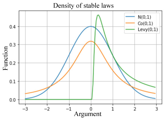
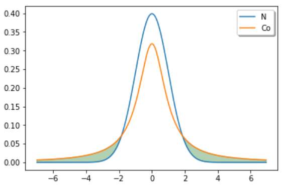
“Heavy tails” are another important feature of sustainable laws (Figure 01 ). It is said that distribution has heavy tails if its residual probability $P(Y>y)$ at the growth of $y$ decreases slower than the indicative distribution $E_1.$This property has been proven for $\alpha <2.$ It can be concluded from this that the property of heavy tails is true for all stable laws, except for the normal ( Nolan, 2017).

Let us show the heavy tails for clarity on the graph implemented on Python 3 for the standard normal law $N\left(\mathrm{0,1}\right)$ and Koshi's distribution $Co\left(\mathrm{0,1}\right)$. Both laws are stable, but the latter has the properties of heavy tails as opposed to the first.

See Full Size >

Student's distribution. Student's Distribution Properties. If ${Z_0,Z}_1,Z_2,\dots ,Z_n$ – are independent standard normal random variables with parameters $\mu =0,{\sigma }^2=1$. Then the distribution of a random variable $t$:

$$t=\frac{Z_0}{\sqrt{\frac{Z_1^2+Z_2^2+\dots +Z_n^2}{n}}}$$

is called the Student's distribution of n degrees of freedom ( Shaw & Lee, 2008).

The Student's distribution (or t -distribution) has a probability density

$$f_n\left(x\right)=\frac{Г\left(\frac{n+1}{2}\right)}{\sqrt{\pi n}Г\left(\frac{n}{2}\right)}{\left(1+\frac{x^2}{n}\right)}^{-\frac{n+1}{2}},\forall x\in R,$$

where G(∙) is an integral of the second kind or gamma function ( Surbhi et al., 2015).

See Full Size >

Previously, in descriptive statistics, the Student's distribution was practically not used as an analytical model. And only relatively recently appeared works in which t-distribution is used to describe the dynamics of various financial indices. The Student's distribution was started relatively recently, as it is "more complicated" than the normal law, because it is not considered to be an asymptotic approximation.

If we talk about the relationship between the Student's distribution and the stable laws of statistics, we can distinguish two properties:

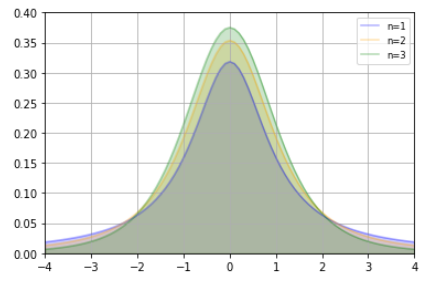
• In case of large degrees of freedom, the Student's distribution converges to the standard normal distribution law, i.e. $n\to \infty t\left(n\right)\stackrel{d}{\to }N\left(0;1\right),$where $\stackrel{d}{\to }$ – distribution consistency

• The Student Distribution with One Degree of Liberty is a standard Koshi distribution $t\left(1\right)=Co\left(0;1\right)$ ( Kremer, 2002)

Then, we can say that t-distribution from both sides is limited by stable laws, from below – by Koshi law, from above – by normal law. And since we consider the Student's distribution as an alternative to the stable laws, it will be reasonable to assume that t-distribution occurs just in those cases when the number of degrees of freedom is not very large and differs from 1.

Purpose of the Study

The purpose of this paper is to identify the relationships and differences between the Student's distribution and sustainable distributions. To show that a statistical process such as a change in the course of a cryptocurrency is subject to the Student's distribution.

Research Methods

To confirm the above facts we will conduct a statistical analysis in Python 3 Jupyter Notebook. To carry out the analysis, we will put forward the main hypotheses and to check them we will use the criterion of Kolmogorov-Smirnov's consent.

Hypothesis statement:

$H_0^1:$ Hypothesis of subordination of XRP (Ripple) course Student distribution for 2018;

$H_0^2:$ Hypothesis of subordination to the normal XRP (Ripple) exchange rate distribution law for 2018;

$H_0^3:$ Hypothesis of subordination of XRP (Ripple) course Koshi distribution for 2018.

The Kolmogorov-Smirnov Consent Criterion is used to test the hypothesis that a sample belongs to a certain distribution law.

Let us suppose that $X_n$– is the original sample, $F_n\left(x\right)$ – empirical distribution function, and $F\left(x\right)$ – theoretical function of distribution of the law assumed in the hypothesis $H_0$.

Statistics of Kolmogorov's criterion is defined as:

$$D_n=\underset{x}{\sup }|F_n\left(x\right)-F(x\left)\right|.$$

Well, then, if the hypothesis is fair $H_0$according to the Kolmogorov's theorem:

$$\forall t>0:\underset{n\to \mathrm{\infty }}{\lim }P\left(\sqrt{n}{D}_n\le t\right)=K\left(t\right)=\underset{j=-\mathrm{\infty }}{\overset{+\mathrm{\infty }}{\sum }}{\left(-1\right)}^j{e}^{-2j^2{t}^2}$$

The hypothesis is rejected if $\sqrt{n}{D}_n$ exceeds the quantile of distribution $K_{\alpha }$ the quantile of distribution $\alpha$, but is accepted otherwise ( Brailov, 2007).

Findings

As the data for the study, we will take the RippleXRP network cryptocurrency rate to the dollar for the period from 01.01.2018 to 31.12.2018.

Upload the data to PythonJupyterNotebook.

See Full Size >

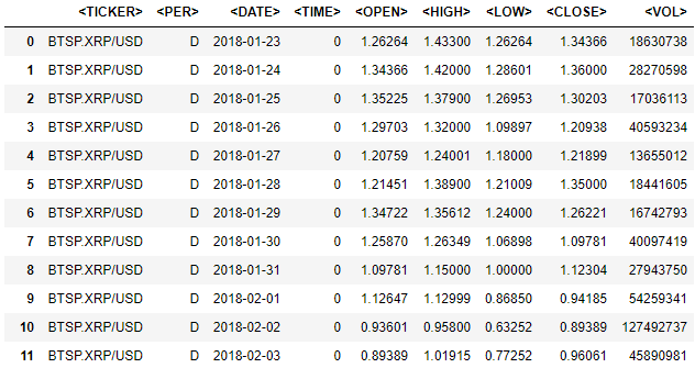
Let us build a histogram of relative frequencies density by closing prices (by column <CLOSE>).

See Full Size >

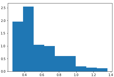
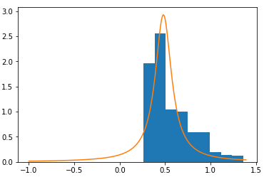
Let us test the hypothesis $H_0^1.$Fig. 5 shows that the histogram is beveled on the right side, so we will select the parameters for the Student's non-central distribution using the fit function.

See Full Size >

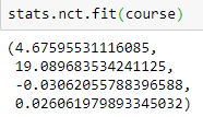
For parameters df=4.67595531116085; nc=19.089683534241125; loc=-0.03062055788396588;scale=0.026061979893345032 superimpose a density graph on the histogram.

See Full Size >

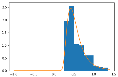
We will run a Kolmogorov-Smirnov test

See Full Size >

The test results show that $\forall \alpha \le 0.09043713341694139$ the hypothesis is accepted. Let us check it out for $\alpha =0.05.$

We have $D_{\mathrm{0,05}}=\frac{\mathrm{1,36}}{\sqrt{344}}=0.07332628577833812$. As $D_{\mathrm{0,05}}>\mathrm{s}\mathrm{t}\mathrm{a}\mathrm{t}\mathrm{i}\mathrm{s}\mathrm{t}\mathrm{i}\mathrm{c}$, is that way, the hypothesis is accepted.

Let us test the hypothesis $H_0^2.$To do this, select the parameters for normal distribution.

See Full Size >

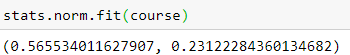
Let us build a normal distribution chart with parameters m=0.565534011627907,σ=0.23122284360134682.

See Full Size >

See Full Size >

Value p value is very small, and we can say that the hypothesis is rejected. Let us check it for the value level $\alpha =0.01.D_{\mathrm{0,01}}=\frac{\mathrm{1,63}}{\sqrt{344}}\approx 0.0878837101608023.$ In this case, the value $D_{\mathrm{0,01}}$ is less than the empirical value of statistics, which means we are in a critical area $K_{\mathrm{0,01}}$. Therefore, the hypothesis is rejected.

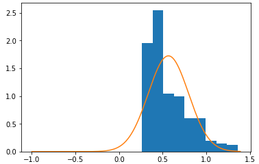
Let us test the hypothesis $H_0^3$о subordination of the XRP course Koshi distribution for 2018. We will select the parameters of Koshi distribution.

See Full Size >

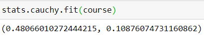
Let us superimpose a graph of Cauchy distribution with parameters a=0.48066010272444215, b=0.10876074731160862 on the relative frequency density histogram.

See Full Size >

We'll run a Kolmogorov-Smirnov test

See Full Size >

Value pvalue it's a small one. It is reasonable to assume that the hypothesis is rejected. Let us check it for the value level $\alpha =0.01$. $D_{\mathrm{0,01}}=\frac{\mathrm{1,63}}{\sqrt{344}}\approx 0.0878837101608023.$ In this case, the value $D_{\mathrm{0,01}}$ is less than the empirical value of statistics, so we are in the critical area $K_{\mathrm{0,01}}$. As a result, this hypothesis is also rejected.

Conclusion

Thus, we come to the conclusion that with the development of different dynamic systems the data cannot obey the normal distribution law, so we have to resort to some alternative variant. The best such variant is the Student's distribution.

Kolmogorov-Smirnov's test has shown that the hypothesis of subordination of the Student's XRP (Ripple) course distribution for 2018 is accepted for $\mathrm{\alpha }\le \mathrm{0.09043713341694139}$, that is, for any significance level below α, the sample will be subject to the Student's non-central distribution law with parameters df=4.67595531116085; nc=19.089683534241125; loc=-0.03062055788396588; scale=0.026061979893345032.

Also by the Kolmogorov-Smirnov criterion we rejected the hypotheses about the subordination of the course to XRP-normal law and the distribution of Koshi, which also shows the need to use the Student's distribution instead of the stable laws of statistics.

References

• Brailov, A.V. (2007). Lectures on Mathematical Statistics. Moscow: Finacademy.
• Daniel, T.P. (2014). A SAS approach for estimating the parameters of an alpha-stable distribution. Procedia Econ. and Finance, 10, 68–77.
• Kremer, N. Sh. (2002). Probability Theory and Mathematical Statistics. Textbook for Higher Schools. Moscow: Uniti-Dana.
• Morozova, M. M., & Pirlik, V.N. (2009). Stable distribution, its modifications and financial derivatives pricing model. Vestn. NGU, 9(1), 97–112.
• Nolan, J.P. (2017). Stable Distributions Models for Heavy Tailed Data. Washington: Amer. Univer.
• Rimmer, R.H., & Nolan, J.P. (2005). Stable Distributions in Mathematica. The Mathem. J., 9(4), 776–789.
• Shaw, W.T., & Lee, K.T.A. (2008). BivariateStudenttdistributions with variable marginal degrees of freedom and independence. J. of Multivar. Anal., 99, 1276–1287.
• Surbhi, S., Harsh, V.S., & Anand, M. (2015). Secure and Robust Watermarking Using Wavelet Transform and Student t-distribution. Procedia Comput. Sci., 70, 442–447.