Adaptive Forecasting Of Work Efficiency Of Agroindustrial Complex Of The Region

Abstract

Modeling a new type of organizational and economic structure of the agro-industrial complex (AIC) of the region is the main task of economic activity in modern Russia. The main problem that arises in modeling AIC indicators of the region is not the stationarity of economic processes in the industry. As a rule, this is connected with the restructuring of AIC industry, the uneven development of scientific and technological progress in the industry, sharp seasonal fluctuations in prices for agricultural products, etc. The economic system in AIC industry is affected by various factors at different times. Thus, the real processes in the industry take place in changing conditions. The model describing the economic system behavior adapts to the series representing this process. Adaptive forecasting methods allow building a class of self-adjusting models of economic systems that are able to reflect the time-varying dynamic processes in AIC industry of the region. The purpose of the work is to study the use of adaptive methods for AIC forecasting of the region. The mechanism of the adaptive model action is shown by the example of efficiency data of AIC work in the region. As an economic series of dynamics, the statistical data on the efficiency work of Lipetsk region are used, namely, the level of profitability, indicators of the technological efficiency of production. Conclusions about the feasibility of a wide application of the adaptive approach for AIC forecasting of the region are drawn.

Keywords: Industrial complexadaptive modelsprofitabilityindicators

Introduction

In recent years, adaptive forecasting methods are widely used by domestic and foreign scientists to verify the models describing economic systems. The use of adaptation principles in economic forecasting was laid at the beginning of the 50s of the 20^th century. The first adaptation models are based on the exponential smoothing method proposed by Brown (1963). Further, foreign scientists were engaged in developments in this area: Box (Box, Jenkins, Reinsel, 2000), Shaw (1984) and others, and native scientists Lukashin and Rahlina (2012), Davnis and Tinyakova (2006), and others (Armstrong, 1989; Chow, 1989; Pesaran, Shin, & Smith, 2001; Cesarno, 1983; Boshoff, 2012; Katsoulacos, 2014).

Problem Statement

The development of the adaptive approach took place in three directions: the first is aimed at increasing the complexity of adaptive predictive models; the second is to improve the adaptive mechanism of forecasting models; the third implements the approach of sharing adaptive principles and other methods of forecasting. The development of models for the joint use of adaptive forecasting and other methods of forecasting is devoted to the works of Levitskii (as cited in Lukashin & Rahlina, 2012), Davnis and Tinyakova (2006). However, the adaptive models were mainly used to forecast financial markets and instruments and are not adapted for economic systems describing real sectors of the economy. Therefore, a need to adapt models to economy sectors, in particular AIC of the region arises.

Research Questions

The subject of the work is modeling AIC activities of the region, using adaptive methods. The sequence of the adaptation process is as follows: at the initial moment of time, the model is in a certain initial state, and the values of its parameters are determined, on the basis of which the prediction is made one step further. After a unit of time is expired (modeling step), the deviation analysis of the effective data of the model from the actual value is carried out (forecasting error). Error data enter the model and rearrange it at the next stage of forecasting, and the whole process repeats at subsequent points in time. Thus, the adaptation is carried out with the receipt of each new actual point of the series. The speed of the reaction depends on the choice of the best adaptation parameter based on the test forecasts of past periods. Adaptive models are flexible enough, but not always universal. Therefore, particular models are built to reflect the dynamics of any specific processes.

Purpose of the Study

The purpose of the work is to study the use of adaptive methods for AIC forecasting of the region; to show the mechanism of action of the adaptive model on the example of data on the efficiency of AIC work in the region (Lipetsk region); to draw conclusions about the feasibility of a widespread use of an adaptive approach for forecasting AIC activity of the region.

Research Methods

The formation mechanism of the model of adaptive expectations

Consider the model

${\mathrm{y}}_{\mathrm{t}}=\mathrm{}\mathrm{}\mathrm{а}+\mathrm{}\mathrm{b}·\mathrm{}{\mathrm{х}}_{\mathrm{t}+\mathrm{1}}^{\mathrm{*}}\mathrm{}+\mathrm{}{\mathrm{\varepsilon }}_{\mathrm{t}}$ (1)

where уt — effective sign value, actual;

х*t+1 — factor sign value, expected.

The mechanism for generating expectations in this model is as follows:

${\mathrm{х}}_{\mathrm{t}+\mathrm{1}}^{\mathrm{*}}-{\mathrm{х}}_{\mathrm{t}}^{\mathrm{*}}\mathrm{}=\mathrm{\alpha }·(\mathrm{}{\mathrm{х}}_{\mathrm{t}}-{\mathrm{х}}_{\mathrm{t}}^{\mathrm{*}})$(2)

or

$\mathrm{}{\mathrm{х}}_{\mathrm{t}+\mathrm{1}}^{\mathrm{*}}\mathrm{}=\mathrm{\alpha }\bullet {\mathrm{х}}_{\mathrm{t}}+(\mathrm{1}-\mathrm{\alpha })·{\mathrm{х}}_{\mathrm{t}}^{\mathrm{*}}\mathrm{}$ (3)

where 0 < α< 1.

Thus, the expected value of xt* factor variable in the period of t is an average arithmetic weighted of its actual and expected values in the previous period. In each period of time t + 1 the expectations are corrected by some fraction α of the difference between the actual value of the factor sign and its expected value in the previous period. The parameter α in this model is called the expectation coefficient. If α tends to 1, the higher the probability of an event, if α tends to zero, this indicates the stability of existing trends. At α = 0 , “conditions prevailing today” will continue for all future periods of time. Expected future values of indicators will coincide with their values of current periods (Shaw, 1984).

Substitute the ratio (3) in the model (1) instead of х*t+1:

${\mathrm{y}}_{\mathrm{t}}=\mathrm{}\mathrm{а}\mathrm{}+\mathrm{}\mathrm{b}·(\mathrm{\alpha }·{\mathrm{х}}_{\mathrm{t}}\mathrm{}+(\mathrm{1}-\mathrm{\alpha })·{\mathrm{х}}_{\mathrm{t}}^{\mathrm{*}})\mathrm{}+\mathrm{}{\mathrm{\varepsilon }}_{\mathrm{t}}\mathrm{}=\mathrm{}\mathrm{а}\mathrm{}+\mathrm{}\mathrm{\alpha }·\mathrm{b}·\mathrm{}{\mathrm{х}}_{\mathrm{t}}\mathrm{}+(\mathrm{1}-\mathrm{\alpha })·\mathrm{b}·{\mathrm{х}}_{\mathrm{t}}\mathrm{}+\mathrm{}{\mathrm{\varepsilon }}_{\mathrm{t}}$ (4)

If model (1) takes place for t period, then it will also occur for period (t-1).

Thus, in the period of (t-1) we have:

${\mathrm{y}}_{\mathrm{t}-\mathrm{1}}=\mathrm{}\mathrm{}\mathrm{а}+\mathrm{}\mathrm{b}·\mathrm{}{\mathrm{х}}_{\mathrm{t}}^{\mathrm{*}}\mathrm{}+\mathrm{}{\mathrm{\varepsilon }}_{\mathrm{t}-\mathrm{1}}$ (5)

Multiply (5) by (1 - α):

${(\mathrm{1}-\mathrm{\alpha })\mathrm{y}}_{\mathrm{t}-\mathrm{1}}=(\mathrm{1}-\mathrm{\alpha })\bullet \mathrm{а}\mathrm{}+\mathrm{}(\mathrm{1}-\mathrm{\alpha })\bullet \mathrm{b}·{\mathrm{х}}_{\mathrm{t}}^{\mathrm{*}}+(\mathrm{1}-\mathrm{\alpha })·\mathrm{}{\mathrm{\varepsilon }}_{\mathrm{t}-\mathrm{1}}$(6)

Subtract term-by-term (6) from (4):

${(\mathrm{1}-\mathrm{\alpha })\mathrm{y}}_{\mathrm{t}-\mathrm{1}}=\mathrm{а}-\left(\mathrm{1}-\mathrm{\alpha }\right)\bullet \mathrm{а}\mathrm{}+\mathrm{}\mathrm{а}\mathrm{}\bullet \mathrm{b}·{\mathrm{х}}_{\mathrm{t}}^{}+{\mathrm{\varepsilon }}_{\mathrm{t}}-(\mathrm{1}-\mathrm{\alpha })·\mathrm{}{\mathrm{\varepsilon }}_{\mathrm{t}-\mathrm{1}}$(7)

or ${\mathrm{y}}_{\mathrm{t}}=\mathrm{\alpha }\bullet \mathrm{а}\mathrm{}+\mathrm{}\mathrm{а}\mathrm{}\bullet \mathrm{b}·{\mathrm{х}}_{\mathrm{t}}^{}+(\mathrm{1}-\mathrm{\alpha })·\mathrm{}{\mathrm{y}}_{\mathrm{t}-\mathrm{1}}+{\mathrm{u}}_{\mathrm{t}}$ (8)

where ${\mathrm{u}}_{\mathrm{t}}=\mathrm{}{\mathrm{\varepsilon }}_{\mathrm{t}}-\mathrm{}(\mathrm{1}-\mathrm{\alpha })·\mathrm{}{\mathrm{\varepsilon }}_{\mathrm{t}-\mathrm{1}}$ .

We obtain an autoregression model, by defining the parameters of which we can easily go to the initial model (1).

Model (1) includes the expected values of the factor variable, which cannot be obtained empirically. Model (8) includes only actual values of variables. Model (1) is called the long-term function of the model of adaptive expectations; it characterizes the dependence of the effective sign on the expected values of the factor characteristic. Model (8) is called the short-term function of the model of adaptive expectations, which describes the dependence of the result on the actual values of the factor.

Findings

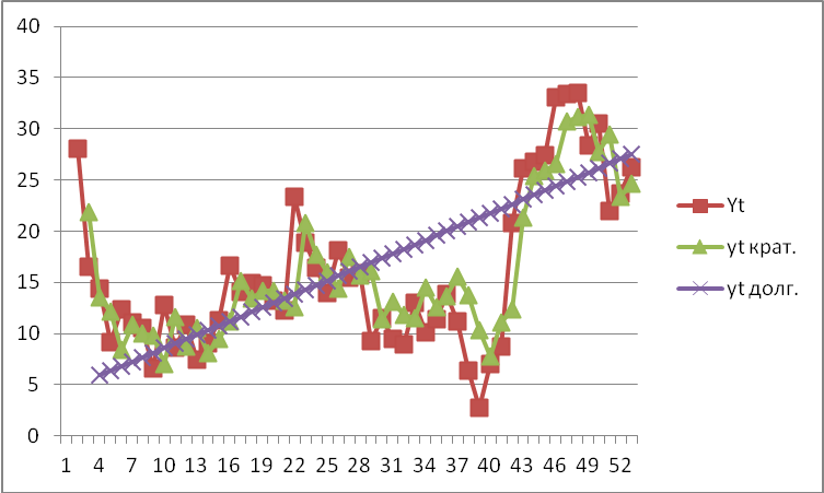
We illustrate the implementation of the adaptive expectation mechanism on the example of data on profitability of agricultural products of Lipetsk region.

Table 1 presents data on the level of profitability of agricultural products sold in Lipetsk region, % (LipetskAdm, 2018).

According to (8) model, we build a short-term model of adaptive expectations, which describes the dependence of the result on the actual values of the factor.

Short-term function of the model of adaptive expectations is $y_t=\mathrm{}\mathrm{1,01}\mathrm{}+\mathrm{0,12}\mathrm{}·\mathrm{}{\mathrm{х}}_{\mathrm{t}}\mathrm{}+\mathrm{}\mathrm{0,73}·\mathrm{}{\mathrm{у}}_{t-\mathrm{1}}\mathrm{}\mathrm{}+\mathrm{}{\mathrm{ս}}_t\mathrm{}$(Fig. 1 ).

Estimate the parameters α = 0,27, b = 0,44, а =3,74 and get the long-term function of the model of adaptive expectations $y_t=\mathrm{}\mathrm{3,74}\mathrm{}+\mathrm{}\mathrm{0,44}·\mathrm{}{\mathrm{х}}_{t+\mathrm{1}}^{\mathrm{*}}+\mathrm{}{\mathrm{\varepsilon }}_t$ (Fig. 1 ).

See Full Size >

Conclusion

It should be noted that the model of adaptive expectations provides accurate long-term forecasts. To improve short-term forecasts, the parameter α in equation (2) must be constantly adapted, since the economic system is not stationary and undergoes constant changes. It is advisable to use the function where α reflects the dependence on any variable, reflecting splashes and declines of AIC industry and the economy as a whole, or a function that reflects the dependence of the calculated and actual data.

The use of adaptive forecasting methods allows us to give an accurate assessment of AIC development of the region and predict its long-term development. Therefore, it is expedient to introduce adaptive forecasting methods to the agro-industrial sector for assessing the activities of the regions.

References

1. Armstrong, J. S. (1989). Combining Forecast: The End of the Beginning or the Beginning of the End?. International Journal of Forecasting, 5(4), 585–592.
2. Boshoff, W. (2012). Advances in Price-Time-Series Tests for Market Definition. Stellenbosh Economic Working Papers: Google Scholar. November.
3. Box, G., Jenkins, G. M., & Reinsel, G. (2000). Time Series Analysis: Forecasting & Control, Wiley-Interscience. New York.
4. Brown, R. G. (1963). Smoothing, Forecasting and Prediction of Discrete Time series. Englewood Cliffs, New Jersy: Prentice-Hall.
5. Cesarno, F. (1983). The Rational Expectations Hypothesis in Retrospect. The American Economic Review, 73(1), 198–203.
6. Chow, G. C. (1989). Rational Versus Adaptive Expectations in Present Value Models. The Review of Economics and Statistics, 3, 71.
7. Davnis, V. V., & Tinyakova, V. I. (2006). Adaptivnyie modeli: analiz i prognoz v ekonomicheskih sistemah. Voronezh: Izd-vo Voronezh. gos. Unta.
8. Katsoulacos, Y. (2014). Quantitative Price Tests in Antitrust Market Definition with an Application to the Savory Snacks Markets. DOI:
9. LipetskAdm (2018). The administration of the Lipetsk region: the official website. Retrieved from: http://admlip.ru/
10. Lukashin, Yu. P., & Rahlina, L. I. (2012). Modern trends of statistical analysis of relationships and dependencies. Moscow: MEMO RAN.
11. Pesaran, M. H., Shin, Y., & Smith, R.J. (2001). Bounds Testing Approaches to theAnalysis of Level Relationships. Journal of Applied Econometrics, 16, 289–326.
12. Shaw, G. K. (1984). Rational Expectations: At Elementary Exploration. New York: St.-Martin’s Press.