
Splinemodels In Forecasting The Balance Of Development Of The Industrial Complex


Abstract
The article covers the possibility and necessity of using splines for analyzing the current dynamics and forecasting stochastic, turbulent and poorly predictable macroeconomic indicators characterizing the balance of industrial development. The essence, advantages, and types of spline modeling as the main research method are analyzed. The expediency of using the spline or spline-polynomial approach in modeling and forecasting the macroeconomic dynamics of the studied balance indicators is confirmed by the formation of a model consisting of successively connected fragments of its change. At the beginning of the study, the selection of the type of spline was made on the basis of a graphic representation of the dynamics of the index of entrepreneurial confidence related to the level of balance in the development of industrial enterprises. It is concluded that correlation splines are most acceptable. Graphic analysis of averaged data of changes in the index of entrepreneurial confidence over the years 2005-2017 allowed to identify 5 fragments describing the annual cycle of changes in the studied indicator. Based on this, the concept of continuous spline approximation of entrepreneurial confidence in the form of a spline-representation of the macroeconomic dynamics of this indicator on the initial discrete set of observation points during the analyzed period has been implemented. The article shows the simplest use of the spline paradigm, which can be extended by a spline approximation of the change in the average value of the index of entrepreneurial confidence during the period studied (2005-2017) in the form of a periodic process.
Keywords: Approximationbalanceentrepreneurial confidenceindustrymacroeconomic dynamicsspline model
Introduction
To assess the state and prospects of development of the industrial complex, it is advisable to describe the current trends of its dynamics and, on the basis of this forecast future changes using economic and mathematical methods. However, this is complicated by the “ragged” nature of the curves of industrial development and the dynamics of its balance in both Russia and other countries.
In this regard, a new tool, an improved research platform is needed to work with indicators of macroeconomic dynamics that characterize the balance of industrial development. Based on the identification and comparison of basic analytical approaches to the study of macroeconomic dynamics, it has been established that fixed-class approximation models cannot accurately describe, analyze and predict financial, economic, production, marketing, and other market processes.
The development of industrial enterprises in the modern period is characterized by periodic, sometimes spontaneous changes in the economic rules of the game: foreign economic relations; economic legislation (norms, tariffs, tax rates, excise taxes, quotas, deductions), as well as organizational regulations, rules, and preferences. Burlachkov (2008) indicates: “an economic system has the property that when external information is incoming its parameters are able to change dynamically”; “Unreasonable government intervention quickly destroys the economic system” (p. 86). In this regard, the required analytical approach must be capable of researching and foreseeing the “ragged” dynamics of real indicators of the economic development of the industrial complex.
Problem Statement
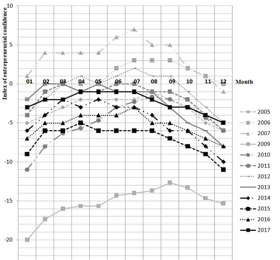
According to research made by Russian scientists (Bezrukova et al., 2017; Parakhina, Boris, & Timoshenko, 2017; Popkova et al., 2017), indicators characterizing the balance of industrial development, such as entrepreneurial confidence, have a “ragged” change character. According to statistics, Russia and other European countries have similar “diseases” of industrial development, leading to the fact that its dynamics change indefinitely and unpredictably (Figures
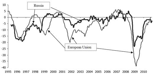
This indicates a lack of confidence in the success of the activity and a low desire to invest in the development of the industry. Although it should be noted as a positive trend, starting in 2015.
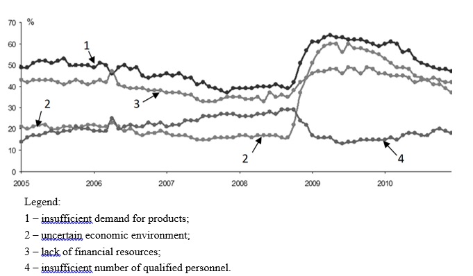
At the same time, most entrepreneurs consider the lack of demand for their products to be the most important reason for which they do not undertake efforts to renovate their enterprises (Figure
This indicates a lack of confidence in the success of the activity and a low desire to invest in the development of the industry. Although it should be noted as a positive trend, starting in 2015.
At the same time, most entrepreneurs consider the lack of demand for their products to be the most important reason for which they do not undertake efforts to renovate their enterprises (Figure
At the same time, the main types of industrial products produce more goods than there is a demand for them (Figure
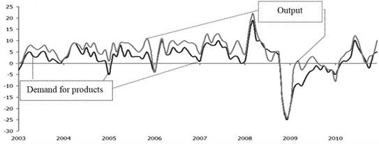
These and other facts show that macroeconomic indicators characterizing the balance of industrial development are stochastic, turbulent, poorly predictable, change spontaneously, quickly, the amplitude of their fluctuations is significant, the variability is significant.
This predetermines the expediency of using the spline or spline polynomial approach in the process of describing, analyzing and forecasting the development of the industrial complex. In this approach, the studied macroeconomic dynamics is represented by a model that includes a set of sequentially related fragments. That is, as the analysis showed, it is advisable to use spline models in such conditions.
Research Questions
-
Are spline models applicable for describing the dynamics and forecasting of economic indicators?
-
What are the conditions for using spline models, their types and forms?
-
What are the advantages of using spline models?
-
What models to choose and how to build them in relation to indicators characterizing the balance of industrial development?
Purpose of the Study
The objectives of the study are:
justification of the use of spline models for describing the dynamics and forecasting indicators of the balance of the economic dynamics of the industrial complex;
formulation of the problem of building a spline model and the formation of an algorithm for its development;
interpretation of the economic meaning of the parameters of spline models and their advantages in describing the dynamics and forecasting indicators of the balance of the economic dynamics of the industrial complex.
Research Methods
As one of the well-known economic and mathematical methods, spline modeling, is proposed as the main research tool, for which a logical comparison of its individual types and an analysis of the features of their use are carried out.
Splines are widely used both in mathematical theory, applied mathematics (numerous computational programs) and in various computer simulation systems.
The theory of interpolation by splines and the term spline itself have found application, primarily, in the works of I. Schoenberg (Schoenberg, 1946).
The name “spline” spline comes from the name of a flexible metal ruler, a universal piece, which was used to connect the points on a smooth curve drawing, which in essence was a graphical interpolation. The “smooth curve” itself, fixed at individual points, is also a spline.
In the problems of approximation, an intuitively similar approach was encountered in mathematics for a long time through the use of spline functions.
The active application of this approach began in the 50-70s of the twentieth century. Currently, for interpolation purposes, splines are traditionally used in computer-aided design systems. However, the potential spline use is much wider than the description of curves of varying complexity.
Splines are an intensively developing field of applied mathematics and econometrics (Wahba, 1990; Pagan & Ullah, 1999; Ruppert, Wand, & Carrol, 2003; Hardle, Muller, Sperlich, & Werwatz, 2004; Keele, 2008). The most widely practical application of splines is found in different branches of physics and related fields (Biggs, Sobolewski, Murry, & Kenny, 2016; Xiao, Liu, Li, Wang, & Zhao, 2016; Shen, Li, Wu, & Zhu, 2017; Pérez-Arribas & Pérez-Fernández, 2018).
Production management objectives are addressed using spline tools, including such issues as optimizing oil production (Jahanshahi, Grimstad, & Foss, 2016), understanding the growth rates of fish catch and fisheries (Chambers, Sidhu, O’Neill, & Sibanda, 2017) and others.
In economic studies, splines have been used to predict the yield curve (Feng & Qian, 2018), credit risk assessments, stress testing and credit asset valuations (Luo, Kong, & Nie, 2016), solving linear quadratic control problems (Yu, Wang , & Li, 2018), to predict stock prices (Rounaghi, Abbaszadeh, & Arashi, 2015), also uses a set of spline rules for predicting business failure (De Bock, 2017).
According to the Soviet scientist Korneichuk (1987), the extensive use of splines in approximation theory for solving the interpolation problem happens due to their good computational and approximative properties, versatility, and simplicity of realization of the models obtained using them.
Another advantage of splines is the efficiency of calculations. However, an excessive increase in the number of fragments and the complication of the functions describing them significantly reduces the advantages of splines as compared to classical approaches.
The definitive characteristic of splines: 1) a spline consists of fragments that represent functions of one class; 2) functions differ only in their parameters; 3) adjacent fragments have docking points; 4) the indicated points of the fragments coincide, ensuring the continuity of the values of the series.
There are a large number of structures called splines. Therefore, it is advisable to use a certain classification in order to choose splines suitable for the task of approximating the indicators characterizing the balance of development of industrial complexes, for example, the index of entrepreneurial confidence.
By designation the splines are grouped into three groups: 1) “interpolation”; the splines of this group pass exactly through the specified points; 2) “smoothing”; these splines pass near the given points, taking into account the errors of their establishment; 3) “correlation”; Splines of this group pass through a set of points and display a certain dependence (trend, regression). According to the key feature, the spline should consist of fragments of the same type, which distinguishes it among other “spline” functions. But at the same time, there are combined splines, which include fragments of various splines. In this case, the main goal is to achieve a given accuracy of approximation with limited time and resources spent on performing calculations. The correct choice of fragments, adequate to the nature of the process, allows increasing the efficiency of calculations.
An important issue is the determination of a sufficient number of fragments. The minimal amount is one fragment. You can build splines with an infinitely large number of fragments, but in reality, these methods and algorithms require a reasonable limit on the number of fragments. Representatives of these splines, as noted by Volkov and Subbotin (2014), are cardinal splines, which were investigated by Schoenberg. Building a model with an unlimited number of fragments is recommended for local splines. When fragments of the same width are available it is possible to calculate the missing parts of the model of the same width. The forecast data can be determined, considering the missing fragments extended to infinity. This allows trend extrapolation.
The functions defining each fragment of the spline depend on a set of parameters, therefore they can change their appearance. The values of the parameters in each fragment are individual and define the shape of a particular spline. For polynomial splines, these are polynomial coefficients, for linear ones – linear ones.
The construction of fragments of a local spline obeys a simple condition: the values of the polynomial at the ends of the segments must be equal to the corresponding value of the interpolated function.
To construct a simple spline – a broken line – this condition is sufficient. The coefficients of a straight line (a fragment of a linear spline) can be determined unambiguously from two equations.
For polynomial splines of higher degrees, additional conditions are required.
At the same time, the extension of such conditions erases the differences between splines and “lumpy” functions.
Findings
To select the type of spline, let us present graphically the dynamics of the index of entrepreneurial confidence (Figure
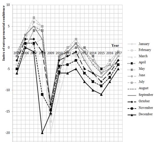
As can be seen from the graph (Figure
As you can see from the presented graphs (Figure
To determine the number of fragments, let us establish the allowable value of the approximation error: in economic calculations, it is 5-10%.
Graphic analysis of averaged data of changes in the index of entrepreneurial confidence over the years 2005-2007, 2009-2017. (Figure
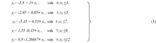
The general formula for linear approximation for each fragment:
where
According to averaged statistical data for 2005-2016 organizations of the manufacturing industry of the Russian Federation received the following model (3):
Calculations showed that the approximation error varies from 0.36% (the second fragment of the spline) to 2.82% (the first fragment of the spline), and in general, is 2.49%, which indicates a fairly high accuracy of the calculations.
When solving forecasting tasks, it is necessary to construct the first forecast fragment in the perspective period so that it is “smoothly” connected (both by the function and all its derivatives) with the last fragment of the period presented in the analysis, if the forward forecasting is performed; with the first fragment of the forecast section in retrospect.
According to experts, there are no restrictions for spline functions in approximation, modeling, analysis, loop search, visualization and forecasting of both periodic and non-periodic macroeconomic processes – there are periodic and non-periodic splines in the theory of splines, and they believe that in the general case the accuracy of approximation non-periodic spline is higher than that of periodic (Vintizenko & Yakovenko, 2008).
Imagine analytics of spline models of macroeconomic indicators of the balanced development of industrial complexes. Spline functions have a high level of analyticity; in its model one can find meaning and characterize analytically, graphically and numerically both the variable S(t) and its derivatives. In mechanics, the first derivative is an impulse, respectively, and in economics, it can be considered an economic impulse obeying the laws of conservation of impulses (Burlachkov, 2008). In analyzing spline models of the balance of industrial development, the first derivative will characterize the speed and direction of its dynamics.
The second derivative in physics is power. The “economic force” acting even in the short section determines the trend (acceleration, deceleration) of economic changes in the entrepreneurial confidence of the industry organizations of the Russian Federation for the period analyzed.
Conclusion
The article uses the concept of continuous spline approximation of entrepreneurial confidence, in which the spline representation of the macroeconomic dynamics of this indicator is most acceptable on the initial discrete set of observation points for the analyzed period. Spline modeling of macroeconomic dynamics has advantages over many approximating functions, including mobility and flexibility of splines, their economy, versatility, visibility of graphical constructions, etc. “Spline-smoothing” is an initial stage in spline modeling, analytics and visual presentation of macroeconomic dynamics.
The article shows the simplest use of the spline paradigm, to which you can add another area of the application – spline approximation of periodic processes, namely, the representation of the change in the average value of the index of entrepreneurial confidence during the study period (2005-2017). The linear part of the spline simulates the trend, and periodic fragments of the spline with parabolic components allow you to simulate the ‘humps” and “troughs” of seasonal or cyclical fluctuations that are quite well expressed in the graphs (Figure
The simplicity of the development and transformation of splines, the high level of reliability of the spline approximation algorithm and the speed of working with it, the multidimensional analytical capabilities of the splines and the visibility of their presentation suggest that splines should be widely used for monitoring, modeling, analyzing cycles and visualizing balance indicators industrial complex development. When using functions of a low degree for modeling fragments of a spline, the economic interpretation of approximation models of individual indicators of balance and its level as a whole is significantly simplified. Approximate spline modeling reflects the dynamics of economic variables, reveals the cyclical nature of changes, increases the accuracy of the subsequent transition to time planning and forecasting indicators of the balance of the industrial complex.
References
- Bezrukova, T. L., Stepanova, Yu. N., Boris, O. A., Savtsova, A. V., Zulpuyev, R. A., & Bezrukov B. A. (2017). Conceptual features of management tools of enterprise structures under the conditions of globalization of the world market. Contributions to economics, 9783319454610, 423-432.
- Biggs, S., Sobolewski, M., Murry, R., & Kenny, J. (2016). Spline modelling electron insert factors using routine measurements. PhysicaMedica, 32(1), 255-259.
- Burlachkov, V.V. (2008). Economic science and econophysics. Economic portal in- stitutionis.com/general/266-2008-06-18-13-45-41.html.
- Chambers, M., Sidhu, L., O’Neill, B., & Sibanda, N. (2017). Flexible von Bertalanffy growth models incorporating Bayesian splines. Ecological Modelling, 355, 1-11.
- De Bock, K. (2017). The best of two worlds: Balancing model strength and comprehensibility in business failure prediction usingspline-rule ensembles. Expert Systems with Applications, 90, 23-39.
- Feng, P., & Qian, J. (2018). Forecasting the yield curve using a dynamic natural cubic spline model. Economics Letters, 168, 73-76.
- Hardle, W., Muller, M., Sperlich, S., & Werwatz, A. (2004). Nonparametric and Semiparametric Models. Berlin Heidelberg: Springer-Verlag.
- Index of entrepreneurial confidence. Industry. Retrieved from https://www.hse.ru/monitoring/buscl/ipu_pp.
- Jahanshahi, E., Grimstad B., & Foss B. (2016). Spline Fluid Models for Optimization. IFAC-Papers OnLine, 49(7), 400-405.
- Keele, L. (2008). Semiparametric Regression for the Social Sciences. Enhland: John Wiley&Sons, Ltd.
- Korneichuk, N.P. (1987). Exact constants in approximation theory. Moscow: Nauka, Main Editorial of Physical and Mathematical Literature.
- Luo, S., Kong, X., & Nie, T. (2016). Spline based survivalmodelfor credit riskmodeling. European Journal of Operational Research, 253(3), 869-879.
- Pagan, A., & Ullah, A. (1999). Nonparametric econometrics. Cambridge University Press.
- Parakhina, V. N., Boris, O. A., & Timoshenko, P.N. (2017). Innovative development of Russian industry: regional problems and opportunities for their solution. Trends of Technologies and Innovations in Economic and Social Studies (TTIESS 2017). Advances in Economics, Business and Management Research, 38, 506-511.
- Pérez-Arribas, F., & Pérez-Fernández, R.A. (2018). B-spline design model for propeller blades. Advances in Engineering Software, 118, 35-44.
- Popkova, E. G., Sukhova, V. E., Rogachev, A. F., Tyurina, Yu. G., Boris, O. A., & Parakhina, V.N. (2017). Integration and Clustering for Sustainable Economic Growth. Springer International Publishing AG.
- Rounaghi, M., Abbaszadeh, M., & Arashi, M. (2015). Stock price forecasting for companies listed on Tehran stock exchange using multivariate adaptive regression splines model and semi-parametric splines technique. Physica A: Statistical Mechanics and its Applications, 438, 625-633.
- Ruppert, D., Wand, M., & Carrol, R. (2003). Semiparametric regression. Cambridge University Press.
- Schoenberg, I.J. (1946). Contributions to the problem of approximation of equidistant data by analytic functions. Part B. On the problem of osculatory interpolation. A second class of analytic approximation formulae. Quarterly of Applied Mathematics, 4(2), 112-141.
- Shen, X., Li, Q., Wu, G., & Zhu, J. (2017). Decomposition of LiDAR waveforms by B-spline-basedmodeling. ISPRS Journal of Photogrammetry and Remote Sensing, 128, 182-191.
- Vintizenko, I.G., & Yakovenko, V.S. (2008). Economic cyclomatics. Moscow: Finance and Statistics.
- Volkov, Yu. S., & Subbotin, Yu. N. (2014). 50 years of the Schoenberg problem on the convergence of spline interpolation. Proceedings of the Institute of Mathematics and Mechanics, Ural Branch of the Russian Academy of Sciences, 20(1), 52-67.
- Wahba, G. (1990). Spline Models for Observational Data. Philadelphia: SIAM.
- Xiao, W., Liu, Y., Li, R., Wang, W., & Zhao, G. (2016).Reconsideration of T-spline data models and their exchanges using STEP. Computer-Aided Design, 79, 36-47.
- Yu, Ch., Wang, Y., & Li, L. (2018).Smoothing spline via optimal control under uncertainty. Applied Mathematical Modelling, 58, 203-216.
Copyright information

This work is licensed under a Creative Commons Attribution-NonCommercial-NoDerivatives 4.0 International License.
About this article
Publication Date
02 April 2019
Article Doi
eBook ISBN
978-1-80296-058-7
Publisher
Future Academy
Volume
59
Print ISBN (optional)
-
Edition Number
1st Edition
Pages
1-1083
Subjects
Business, innovation, science, technology, society, organizational theory,organizational behaviour
Cite this article as:
Parakhina, V., Timoshenko, P., Simonov, A., & Chernyshov, M. (2019). Splinemodels In Forecasting The Balance Of Development Of The Industrial Complex. In V. A. Trifonov (Ed.), Contemporary Issues of Economic Development of Russia: Challenges and Opportunities, vol 59. European Proceedings of Social and Behavioural Sciences (pp. 657-667). Future Academy. https://doi.org/10.15405/epsbs.2019.04.70