
Modified Method Of Real Options: Evaluating R&D Projects


Abstract
The study reveals the problem of estimating the value of R&D projects that are considered as a two-stage process, during which a company makes two types of investments: an initial investment (purchase of an option) and a subsequent investment (exercise of an option). The value of an R&D project is determined by the option to invest in future business exploitation and the expected future cash flows from the commercialization of the R&D results. The authors of the article also note such R&D features as: large time periods between basic research and the commercialization of the results; high uncertainty of the cost and income; the need to take into account legislative regulation in the field of standardization and licensing. Due to the R&D projects’ features, when applying the method of discounting cash flows during evaluating the R&D projects, uncertainty and, consequently, the degree of flexibility in management decision-making process, are not taken fully into account. Hence, the value of an R&D project is underestimated. The paper proves the expediency of using the method of real options in conjunction with the theory of games. To carry out a reliable valuation of R&D projects, the authors propose to use a complex model, created using the real options method with an integrated Poisson jump process. This made it possible to evaluate the option value of R&D projects, considering the possibility of “technical failure” at each stage of the project. This model is particularly effective in high-tech industry.
Keywords: Real optionsvaluevaluationR&DPoisson jump processDCF
Introduction
The question of turning Russia into one of the global leaders of the world economy requires a focus on the R&D projects. Improving the effectiveness of R&D seems to be a difficult task without a well-functioning system of financing and valuation. The value of R&D is not a typical task, since such projects are of a high level of uncertainty and consist of a combination of various risk factors. The widespread DCF-method is not an appropriate method to value R&D projects. The most acceptable is the method of real options that considers various kinds of uncertainties. At the same time even if we use method of real options, we have to take into account additional elements, to get a reasonable result. R&D projects can be viewed as an option to expansion suggesting the possibility of moving from one research stage to another after successful completion of preceding stages. In the context of corporate finance, this is a managerial flexibility and this factor has a certain value; but in the context of real options method, this flexibility takes the form of a compound call option. In essence, compound options are a combination of options, in which the exercising of one option creates favourable conditions for appearance of another option. For the first time, compound options began to be used to evaluate sequential investment opportunities. Geske (1979) demonstrated that securities with the sequential pay-outs could be valued as compound options. Carr (1988) analyzed compound option as an option to acquire a sub sequential option that allows the exchange of one asset for another. Lee and Pakson (2001) applied Carr’s compound exchange option formula for R&D project valuation. A compound option may be applied in many industries, especially for estimating value of R&D projects in a high-tech sector of the economy – the projects implemented in these industries consistently create real options both on continuing research and implementing the results of developments, and on their cancellation due to adverse outcomes. As a result, in the budgeting process of capital investments, the pricing model of compound options began to be applied to determine the value of R&D projects. So, Shockley, Curtis, Jafari, & Tibbs (2003) were the first researches who adapted a multi-stage binomial option pricing model for estimating the value of R&D in biotechnology sector. Cassimon, Engelen, Thomassen, & Van Wouwe (2004) derived the equation in closed-ended form for an N-nested compound option and successfully implemented it to estimate the value of an application for approval and registration of a new drug in the US. These studies do not make a clear distinction between the technical and economic uncertainty - it is implied that the uncertainty is one-dimensional, and the base value is modelled by means of a geometric Brownian motion. The exception is the study of Copeland and Antikarov (2001), who simulated two types of compound R&D options and use the binomial lattice method to estimate the value. The key value of this study is that the authors differ the technical and economic uncertainties and estimate their effect on the project value using the quadrinominal approach.
Problem Statement
Because of the nature of the R&D projects, it would be incorrect to use standard valuation methods and tools. Thus, there arises a necessity to develop new methods and tools to estimate the R&D projects value.
To achieve the purposes of this paper, it is necessary:
To analyse the evaluating subject’s features and the types of options
To analyse the features of different types of real options and select the option that is to R&D project and reveal the essence of the R&D option
To analyse the Poisson jumps and the diffusion process and the expediency of its use for modifying the method of real options
Determine the set of risks of an R&D project
To study how the R&D option value creates and estimate its value under the different scenarios that consider occurrence of the technical failure.
Research Questions
The study aims to answer the following questions:
How to estimate the value of R&D projects?
What are the methods we can use to better estimate the R&D projects value?
Purpose of the Study
The purpose of this study is to deepen the distinction between technical and economic uncertainty and demonstrate how they relate. In contrast to Copeland and Antikarov (2001), we simulate compound real options, where the flows of new information occur both continuously and abruptly. The goal is also to prove that the pricing model of a standard compound option provides the necessary tools to estimate the value of an R&D project in a high-tech sector, since it does not allow only technological uncertainty to be taken into account. The model assumes that there is a positive probability that the project has an unfavorable outcome in the event of technical failure. It also assumes that at each point of time it follows the Poisson distribution, so combining the Poisson jumps and the diffusion process, we can study a compound R&D option that provides the possibility of abandoning further project implementation at each stage of development.
Research Methods
Methods: analysis and synthesis method; abstraction method, modelling, simulating of a diffuse-jump model, case analysis.
Findings
Determining the value of an R&D project is a non-standard task, since such projects have a high degree of uncertainty and sets of various risk factors. The DCF-method can be limitedly applied to the valuation of these projects. The most acceptable is the method of real options, which considers the various uncertainties, but even if this method is applied, additional elements must be taken into account to obtain a reasonable project value. The R&D projects can be viewed as an option to expand suggesting the possibility of moving from one research stage to another only if favourable opportunities are given. In terms of corporate finance, this is a trivial managerial flexibility and given factor has a certain value. In terms of Real Options method, this flexibility has the form of a compound call option. In essence, compound options are a set of options, where the exercise of one option leads to the emergence of another option.
The main objective of this paper is to make a deeper distinction between the technical and economic uncertainty and demonstrate interaction between them. In contrast to Copeland & Antikarov (2001), we construct a model of compound real options, in which the flow of new information occurs both continuously and abruptly. We also conclude that the pricing model of a standard compound option provides the necessary tools for estimating the value of R&D projects in the pharmaceutical sector, since it does not allow to take into account only technological uncertainty. Our model assumes a positive probability that the project has an unfavourable outcome in case of technical failure (Bernstrom, 2014). The probability of an unfavourable outcome at each point in time follows the Poisson distribution. By combining Poisson jumps and a diffusion process, we can explore a compound R&D option that provides an opportunity of abandoning further project implementation at each development stage. The practical applicability of the jump-diffusion model of a compound option that we developed is confirmed by using the case analysis method (Copeland & Copeland, 2003).
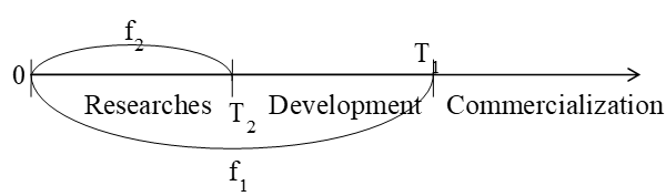
In this study, for clarity, we use a call option for a call option with two strike prices and two maturity dates. The main assumption of our model is that at time 0 (the beginning of the basic research stage), the pharmaceutical company acquires an option on R&D of a new drug by investing the amount I2 (the strike price of a compound option) at the date of expiration T2. If this stage completes successfully, the company acquires another option for commercialization by investing the amount I1 (the strike price of option) at the date of expiration
The main state variable in our model is the present value of all future cash flows (hereinafter referred to as “R&D value”) obtained at time t and followed the jump-diffusion process. Pennings and Lint (1997), Martzoukos and Trigeorgis (2002), Wu and Yen (2007) also consider models for estimating the value of R&D using the Poisson process, in which a finite number of jumps can influence the value of a basic project in each time period and in which the sizes of these jumps are stochastic. Experiments simulated according to the Poisson process include such elements as competition, judicial practice in the field of patent protection, etc. Regarding the project in the pharmaceutical sector, we model the emergence of new information in accordance with the Poisson process, assuming the implementation of only one jump in each time interval. In our model, the jump represents unfavourable outcome of the project. Therefore, the size of the jump is taken as a constant and is not stochastic (Benninga & Tolkowsky, 2002).
Below we specify the project value dynamics in terms of the technical risk of an unfavorable outcome. For clarity, the process of constructing a simplified jump-diffusion model, we begin with the basic jump-diffusion model.
The value of the project remains uncertain during many development stages. Denoting Vt (where t [0, T1]) as a project value, we assume that Vt follows log-normal jump-diffusion process. The value of the basic project, represented by the jump-diffusion model, has two sources of uncertainty: diffusion risk σdzt (typical for an ordinary company), which includes positive and negative random fluctuations, and the condition dqtt, which describes the emergence of major jumps leading to sharp increases/decreases in a value. On average, in the time frame [0, t] we see λt jumps, average relative size of jump is E[Y-1] and the number of jumps is not dependent on their size or other uncertainty indicated in the model.
For the purpose of valuation of R&D project, we use a simplified version of the jump- diffusion model, where Y is not a stochastic value and is not observed or observed the only one jump in the project value in a time frame with a duration t. Thus, the jump-diffusion model has the following form:
(1)
where:
α – expected rate of return of the project;
σ – standard deviation of the project;
zt – standard Brownian motion process;
V0 – the present value of the base project;
φt – the indicator of technological uncertainty describing the probability of project success. In a more particular case, this is an exponential Poisson random variable nt (independent of zt) with a parameter λ (>0), which describes the probability of jump occurrence and a deterministic parameter ln(Y), showing amplitude jump. Particularly:
In this study we assume that only one single jump is possible (nt=0 or nt=1) and if such a jump takes place, the project depreciates completely. Thus:
And its expected value is
We assume that the company is risk neutral, therefore, replacing the expected rate of return α in (1) with α = r + βσ, where r is a risk-free rate of return (r ≥ 0) and β is a market price of diffusion risk, the equation for calculating the terminal value of the project Vt can be represented as follows:
where z* = z + βt is a new Brownian motion process in a risk-neutral environment, z* and nt are variables that are independent of each other as we indicated above.
It should be noted that the jump does not correlate with the major changes in the economy. It represents an idiosyncratic risk that can be diversified and has a zero risk market value.
Risk neutrality means that the weighted average of the project's present value with a zero jump and with a single jump equals to the future value of the project and can be calculated by dividing of the present value of the project by the expected value of the jump. Consequently,
which implies that the deterministic movement of the process (1) is replaced by the risk-neutral movement (r + λ - σ2), where λ is a compensation for the risk of a technical jump in the time frame [0, t]. Due to the fact that the rational investors will not invest in assets that have insufficient profitability, it must be compensated for the risk of an additional jump.
An R&D option value is evaluated based on the assumption that its value at any time in the future t is determined by two possible scenarios: an unfavourable outcome occurs or does not occur. Consider Vt | (nt = 1) as the terminal value of the project, provided that the technical failure occurs in the period [0, t]. This can be expressed as follows:
(2)
and its expected value is:
Further, consider Vt | (nt = 0) as the terminal value of the project, provided that the technical failure does not occur in the period [0, t]. Then the value equals:
(3)
The expected value of Vt | (nt = 0) equals:
We assumed that the information about success or failure appears in the end of each stage. Consequently, each investment option will be exercised in the case of successful completion of preceding stage.
Consider the problem of evaluating an option of launching a product to the market at time zero. T1 is time of launching a product, as a result appear commercialization cost I1, – is a project value. The gain from the project at time T1 will be max{ - I1, 0}. The value of an investment opportunity at time t denote as F1 (V, t). If the value V at time T1 is higher than I1, the product will be introduced to the market, that is, the option will be exercised, otherwise the option will not be exercised.
The value of this investment opportunity at time zero equals to the expected present value of the cash flows:
The estimation of the investment value F1 (V, 0) with jumps is not a difficult task. Consider n as a number of jumps that takes place in the time interval with the length of T1. The appearance of a jump reduces the value of the project to zero and the random variable n equals to zero with probability or equals to one with probability 1 - . Based on two scenarios, we can calculate F1 (V, 0) as a weighted sum of the prices of call options, provided that the technical failure occurs or does not occur:
(4)
The value of the first part of expression (4) can be easily calculated. Based on the fact that the technical failure occurs, the terminal value of the project at the point in time T1 is
| (n = 1) = 0. This can be derived by applying formula (2). Thus, the expected terminal value of the option: – has no value because profit equals to zero.
Consider the second part of expression (4). The terminal value of the project in the case of absence of the technical failure is:
Estimation of the value of a single call option with a jump to zero risk is reduced to the calculation of the value of a single call option with an increased discount rate:
Thus,
(5)
where is a cumulative standard normal distribution, h1 and l1 equal to:
Equality (5) is similar to the Black-Scholes call option pricing formula, considering that the technical failure does not occur during the life of the option and it is weighted with the probability of zero technical risk. The equals to the present value of the future cash flows, depending on the project outcomes and the exercise of the option, and the can be interpreted as the present value of the payment with the strike price I1.
Consider valuation of a compound R&D option, which at time T2 gives the enterprise the right to purchase another option (basic option) for I2, with the strike price I1, and the exercise date T1. At time T1 the underlying (basic) option gives the right to launch a product to the market. The value of the compound option at time T2 is:
where F1 is the value of a simple call option at time T2 with the exercise price I1 and the expiration date T1 = T2 + . Hence, if at time T2 the value of the option is greater than the exercise price I2, the compound option will be exercised, otherwise, it will not.
The value of the compound option at time zero equals to the expected present value of the cash flows:
The valuation of this option requires taking into account two possible scenarios, namely, the scenario in that a failure occurs in the time interval [0, T2] and the scenario in that the failure doesn’t occur in the time interval (T2, T1]. Let n2 and n1 are the number of jumps that occur in the intervals [0, T2] and (T2, T1], therefore ( = T1 - T2). Thus, the random variables n2 and n1 are the Poisson variables with probabilities and , respectively, if the failure does not occur, and 1 - and 1 - if it occurs.
Knowing that F1 can be calculated using equation (5), then,
where:
As a result, the value of a compound option at time zero is:
(6)
If the technical failure occurs in the interval [0, T2], then the conditional value of the project at time T2 equals:
and, accordingly, the expected total value of the compound option [max {F1 - I2, 0}| n2 = 1] is lost because its value is equal to zero.
On the other hand:
is the terminal value of the project at time T2, based on the assumption that the technical failure does not occur in the time interval [0, T2], then:
which equals to:
where n (.) is a normal density function, , function can be represented as:
and the constant is determined by the equality:
The value of the compound option at time zero is equal to:
(7)
where:
Factor is a function of standard bivariate normal distribution with the correlation coefficient , and is the critical value of the project, such that the underlying (basic) option’s value at time T2:
then
In accordance with (7) the pricing formula is similar to the pricing formula of a compound Heske option, provided that the technical failure weighted with the probability of a zero technical failure does not occur in the intervals and the expression can be interpreted as the present value of the possibility of obtaining future cash flows, which depends on the success outcome of the stages of research and development, and the execution of both a compound and basic option.
The study shows that R&D project can be realized as a series of projects, where investment decision relies on the successful completion of the preceding R&D stages. Before the R&D results (developments) become a good and starts its selling, there is no cash flow generation. This particular R&D projects’ feature turns into a difficult task the R&D project valuation. Unlike the DCF-method, which is not fully applicable to value the R&D projects, the method of real options provides an expanded set of valuation models, each of which focuses on the specific project features (Damodaran, 2007).
The models of compound options, with the presence or absence of technical failure, have not been studied previously. Introducing the Poisson jump process into the method of real option, we estimated the option value of R&D project, taking into account the possibility of technical failure at each of the project stages. Our method has demonstrated that a compound R&D option can be valued based on two possible scenarios: a technical failure occurs and does not occur. When the technical failure occurs, the investment option is rejected, therefore, the task is reduced to estimating the value of a compound R&D option with favourable outcome.
The practical applicability of this model has been tested using case analysis.
We evaluated R&D project considering a positive probability of the technical failure and vice versa. The sensitivity analysis results showed that both types of uncertainty have a positive effect on the value of the R&D option. We found that the sensitivity of the value of the option to the volatility of the base value and the cost of commercialization reduces in case of presence of technical uncertainty.
The method we showed is applicable for evaluating sequential investments opportunities in R&D projects in those industries in which there is a positive likelihood of technical failure at various stages of the project. Our model can be extended with an arbitrage complexity for N-nested compound options. Such a model will be very efficient in evaluation of R&D projects at early stages.
Conclusion
1. Estimation of the value of R&D projects is significantly different from the valuation of other objects, because a high degree of uncertainty and a combination of various risk factors are inherent to such projects.
2. The widespread DCF-method can be limitedly applied for R&D projects valuation. The most acceptable one is the method of real options that takes into account various kinds of uncertainties, but to obtain a reasonable value, more additional elements must be considered.
3. It is better to consider R&D projects as an option to expand suggesting the possibility of moving from one stage to another only after the successful completion of preceding stages. This managerial flexibility has a certain value; in terms of real options, this flexibility has a compound call option form.
4. During the study several relations have been identified:
An increase in the value of a basic project leads to an increase in the value of a compound option
The increase in the volatility of the basic project cost causes an increase in the value of a compound option
An increase in the average annual commercialization expenditures leads to an increase in the value of a compound option.
Acknowledgments
This research completed as the part of the State task of Financial University in 2018.
References
- Benninga, S.Tolkowsky, E. (2002). Real options—an introduction and an application to R&D valuation.. The Engineering Economist, 47(2), 151-168
- Bernstrom, S. (2014). Valuation: the market approach. : 637-654
- Carr, P. (1988). The valuation of sequential exchange opportunities.Cassimon, D., Engelen, P. J., Thomassen, L., & Van Wouwe, M. (2004). The valuation of a NDA using a 6-fold compound option. Research Policy, 33(1), 41-51.Copeland, T., & Antikarov, V. (2001). Real Options: APractitioner’s Guide, NewYork, NY: W.W. Norton & Company Copeland, T., & Copeland, T. E. (2003).. Real Options, Revised Edition: A Practitioner's Guide, 43(5), 1235-1256
Copyright information

This work is licensed under a Creative Commons Attribution-NonCommercial-NoDerivatives 4.0 International License.
About this article
Publication Date
20 March 2019
Article Doi
eBook ISBN
978-1-80296-056-3
Publisher
Future Academy
Volume
57
Print ISBN (optional)
-
Edition Number
1st Edition
Pages
1-1887
Subjects
Business, business ethics, social responsibility, innovation, ethical issues, scientific developments, technological developments
Cite this article as:
Tazikhina, T., Grúzin, A., & Fedotova, M. (2019). Modified Method Of Real Options: Evaluating R&D Projects. In V. Mantulenko (Ed.), Global Challenges and Prospects of the Modern Economic Development, vol 57. European Proceedings of Social and Behavioural Sciences (pp. 931-941). Future Academy. https://doi.org/10.15405/epsbs.2019.03.92