
Modeling And Forecasting Financial Performance Of A Business: Statistical And Econometric Approach


Abstract
By employing statistical methods, econometric modeling and forecasting financial indices this study attempts to analyze financial performance of a typical Russian company operating in consumer goods industry. Financial data for analysis has been obtained in the statements of the company for 2016-2018 and are presented as monthly time series. The approach to empirical research adopted for this study is a mixed time series methodology based on methods to detect trends and abnormal observations, tests for stationarity, graphical analysis of autocorrelation function and partial autocorrelation function, methods of constructing and assessment of econometric models, and the comparison of forecast capabilities of constructed models. This research offers multiple regression model of dependence of profit on other financial indices. To forecast profit and other indices autoregressive moving average model is also examined in this study. Constructed models were applied to test forecasts of profit. The findings demonstrated the advantages of forecasting based on multifactor linear regression model. The point and interval forecasts for upcoming period are presented. The findings of this study demonstrate that there is no positive dynamics of monthly profit, however, there is no risk of bankruptcy as well. The second major finding was that the negative influence of increased net cost, decreased production and sales volumes could cause the decrease in profit during the period forecasted.
Keywords: Financial performanceprofiteconometric modelforecastingtime series
Introduction
Russian businesses have faced the whole range of challenges: harsh competition, imperfect tax system, financial instability, and risk of bankruptcy. This environment is where a business “bears full responsibility for its activities to its shareholders, employees, banks and investors” (Sakayeva, Iremadze, & Grigorieva, 2010, р. 78). Thus, there is an urgent need for any business to constantly monitor its financial status and the efficient use of its resources.
Monitoring events depend on a business type and on the system of indices that characterize its financial status (Strokovych & Mykolenko, 2018; Dikareva & Kankhva, 2016) or financial resilience (Bidzhoyan & Bogdanova, 2016; Khudyakova & Shmidt, 2015), on bankruptcy probability assessment (Temchenko & Kryshtopa, 2017), on economic sustainability assessment methods (Khudyakova & Shmidt, 2015), and on competiveness assessment (Borodin, 2015), etc.
Problem Statement
Profit is the major indicator that characterizes financial result of business activities. Having profit allows a firm to pay its investors and suppliers, to pay taxes, to expand the range of products, and to upgrade its equipment (Sakayeva, Iremadze, & Grigorieva, 2010).
An application of econometric and statistical methods to a thorough analysis of profit could enable a business to adjust its plans and take rational managerial decisions.
This paper analyzes the financial indices of a limited liability company ‘Samarsky Trikotazh’. This company is listed in Russian small and medium size company register. The company is listed as a micro business and is seen as a typical company of a consumer goods industry. The core activity of the company is production and wholesale of knitted and jersey goods.
The data for the research in question were taken from financial statements of the company. The indices analyzed illustrate financial resilience of the company. Preliminary statistical analysis allowed us to select the following indices (thousands of rubles): Y- monthly profit, X1 - production price, X2 - general and administrative expenses, X3 - revenue. The data represent monthly time series dynamics for the period from January 2016 to April 2018. Statistics and data were analyzed with MS Excel, Gretl, Eviews software.
Research Questions
The research attempts to fulfill the following tasks:
to carry out preliminary statistical analysis of financial resilience indices;
to construct econometric models of profit and other indices under research;
to compare forecasting potential of the models constructed;
to make a point forecast and an interval forecast of profit for upcoming periods.
Purpose of the Study
The aim of this paper is to construct econometric models of financial resilience indices and to forecast profit through the best selected model. The profit is seen as a financial result of a firm’s operational activity.
Research Methods
There are a number of studies which utilize different approaches towards economic indices modeling and forecasting. Among others profit indices have been explored. Gadelshina and Aksyanova used multitrend models to forecast profit (Gadelshina & Aksyanova, 2013). Sukhova (2012) explored profit forecasting based on autoregression models and adaptive expectation models. In (Klebanova & Rudachenko, 2015) to forecast bankruptcy adaptive models were used.
The methodological approach taken in this study is a mixed methodology based on time series of selected financial indices: methods for detection trends and abnormal observations, stationarity tests, graphical analysis of autocorrelation function and partial autocorrelation function, methods of econometric models construction, model residuals tests for heteroscedasticity and autocorrelation, and methods for comparison the forecasting resources of econometric models.
Findings
The construction of econometric models was preceded with the statistical analysis of all the indices under study.
Analyzing time series of financial indices it is important to identify the pattern of their time dynamics and their development trends.
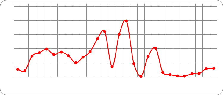
Time series graph of the indices revealed instability in the dynamics of the changes. Figure
Foster-Stuart test was applied to reveal the trend of financial indices presence in time series. The results are shown in Table
To test the homogeneity of index sets their statistical characteristics were calculated. In comparison to 2016 in 2017 an average monthly profit (
The analysis revealed that the

where,


Test values

After the conversion of
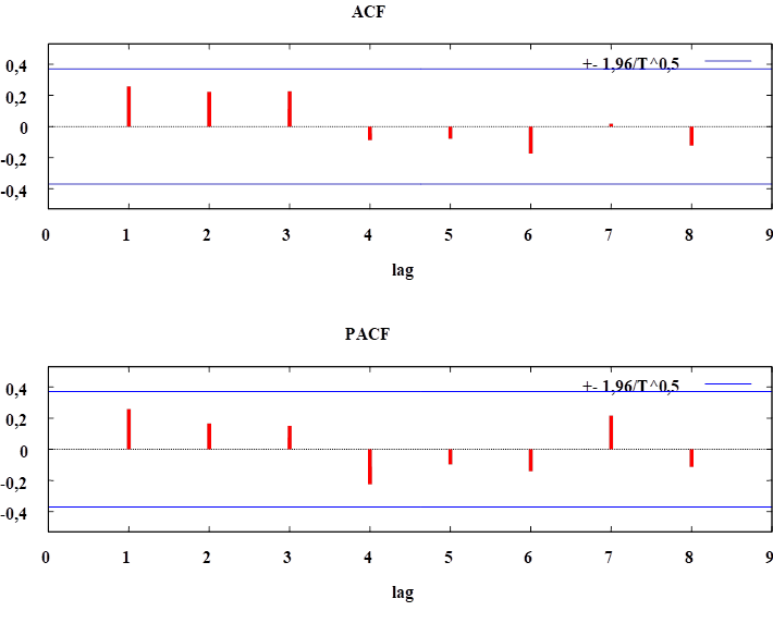
Testing for time invariance is an essential stage when a time series econometric model is developed. Initial data graphs were analyzed to test the time invariance of indices under study. The graphs of autocorrelation function (ACF) and partial autocorrelation function (PACF) were also studied. The results of augmented Dickey-Fuller test (ADF-test) were considered (Derunova, Ustinova, Derunov, & Semenov, 2016). Table
Two types of econometric models were constructed in this study. First, the model was adjusted to the time series of every index. Time series of all indices under study were invariant and were described with autoregression processes and moving average (

Time series of other indices are best described with

In models (2) and (3):


The results of time series modeling are shown in Table
Thus, for

The constructed
Having a good forecasting capability, which their major task is,

Tentatively, to find and exclude multicollinearity from the model (5) a matrix (Table
From the matrix it is apparent that there is no multicollinearity among the explanatory variables (indices
To assess the parameters of the model (5) least squares method (LSM) was applied. The results are shown in Table
Thus, the constructed model of monthly profit has the form:

According to the simulation results, model parameter estimates are significant at 5% significance level (except the intercept). In general the model is also significant (the experimental value of
The constructed model shows that one thousand rubles increase in net cost is followed by an average 0,96 thousand rubles decrease in profit; 1 thousand rubles growth of general and administrative expenses decreases monthly profit by 1,1 thousand rubles; the revenue growth increases monthly profit by 0,99 thousand rubles on average.
Regression residuals analysis of the constructed model (6) demonstrated their stationarity (
Test forecasting of


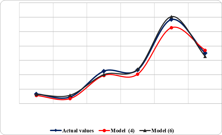
To compare the accuracy of forecast among the models tested the mean relative forecast error was calculated:

where


Constructed multifactor regression model (6) was applied to develop point and interval forecasts (Wilke, 2018) for monthly profit of LLC ‘Samarsky Trikotazh’ for upcoming months of 2018. The first step of the profit forecast included the calculations of values for
The findings showed the following profit forecast values for October, November, and December 2018:


The current research has revealed that the profit forecasted demonstrated the tendency to decline.
Conclusion
The findings of this study demonstrate that there is no positive dynamics of monthly profit, however, there is no risk of bankruptcy as well. The second major finding was that the negative influence of increased net cost, decreased production and sales volumes could cause the decrease in profit during the period forecasted. The research has also shown that the constructed models are reliable and their quality is sufficient to forecast monthly profit and other financial indices.
The research of company financial resilience would be a fruitful area for further work. Several questions still remain to be answered. Methods of assessing bankruptcy probability should be examined with logit models or other binary and multiple choice models.
References
- Bidzhoyan, D.S., & Bogdanova, T.K. (2016). Modelling the financial stability of an enterprice taking into account macroeconomic indicators. Business Informatics, 3(37), 30-37. DOI:
- Borodin, A.I. (2015). The concept of the mechanism of management in the financial potential of the enterprise. Tomsk State University Journal, 391, 171-175. DOI:
- Derunova, E.A., Ustinova, N.V., Derunov, V.A., & Semenov A.S. (2016). Modeling of Diversification of Market as a Basis for Sustainable Economic Growth. Economic and Social Changes: Facts, Trends, Forecast, 6, 91-109. [in Rus.]
- Dikareva, V., & Kankhva, V.S. (2016). Evolution Procedure for Financial Stability of the Enterprises of Housing and Utilities Infrastructure. In International Science Conference SPbWOSCE – SMART, 106(8022). DOI: 10.1051/matecconf/20171060 SPbWOSCE-2016 8022
- Gadelshina, G.A., & Aksyanova, A.V. (2013). Forecasting of company’s profit with multitrend model. Bulletin of Kazan Technological University, 16(1), 277-281. [in Rus.]
- Khudyakova, T.A., & Shmidt, A.V. (2015). Methodological Approach to Forecasting Financial and Economic Enterprise Stability. In K.S. Soliman (Ed.), Innovation management and sustainable economic competitive advantage: from regional development to global growth: Proceedings of the 26th International Business Information Management Association Conference (pp. 1612-1616). Madrid: International Business Information Management Association.
- Klebanova, T.S., & Rudachenko, O.O. (2015). Forecasting the Indicators of Financial Activities of Housing and Communal Services Enterprise Using Adaptive Models. Buziness Inform, 1, 143-148.
- Sakayeva E., Iremadze, E., & Grigorieva, T. (2010). Forecasting and analysis of factors of financial sustainability of an enterprise on the basis of mathematical modeling. Bulletin MRSU. Series: Economics, 3, 78-88. [in Rus.]
- Strokovych, H.V., & Mykolenko, O.P. (2018). Formation of the system of assessments of the financial and investment potential of an enterprise. Financial and credit activity-problems of theory and practice, 2(25), 246-252.
- Sukhanova, E.I., & Shirnaeva, S.Y. (2015). Different approaches to macroeconomic processes simulation and forecasting. Fundamental Research, 12, 406-411. [in Rus.]
- Sukhanova, E.I., Shirnaeva, S.Y., & Mokronosov, A.G. (2016). Econometric models for forecasting of macroeconomic indices. International Journal of Environmental and Science Education, 11(16), 9191-9205.
- Sukhova, N.A. (2012). Mathematical modeling of sales revenue with econometric methods. Intellectual potential of XXI century: stages of knowledge, 9(2), 192-197. [in Rus.]
- Temchenko, O.A., & Kryshtopa, I.I. (2017). Substantion for mining and concentrating enterprises` financial stability based on integral bankruptcy indicators. Financial and credit activity-problems of theory and practice, 2(23), 241-250.
- Trofimenko, S.V., Marshalov, A.J., Grib, N.N., & Kolodeznikov, I.I. (2014). Modification of the method for Irwin detect abnorval levels time series: method and numerical experiments. Modern problems of science and education, 5, URL: http://science-education.ru/ru/article/view?id=15130 (accessed 30 September 2018). [in Rus.]
- Wilke, R. A. (2018). Forecasting Macroeconomic Labour Market Flows: What Can We Learn from Micro-level Analysis? (2018). Oxford Bulletin of Economics and Statistic, 80(4), 822-842.
Copyright information

This work is licensed under a Creative Commons Attribution-NonCommercial-NoDerivatives 4.0 International License.
About this article
Publication Date
20 March 2019
Article Doi
eBook ISBN
978-1-80296-056-3
Publisher
Future Academy
Volume
57
Print ISBN (optional)
-
Edition Number
1st Edition
Pages
1-1887
Subjects
Business, business ethics, social responsibility, innovation, ethical issues, scientific developments, technological developments
Cite this article as:
Sukhanova, E., Shirnaeva, S., & Zaychikova, N. (2019). Modeling And Forecasting Financial Performance Of A Business: Statistical And Econometric Approach. In V. Mantulenko (Ed.), Global Challenges and Prospects of the Modern Economic Development, vol 57. European Proceedings of Social and Behavioural Sciences (pp. 487-496). Future Academy. https://doi.org/10.15405/epsbs.2019.03.48