The First Acquaintance Of Schoolchildren With Hard Programming Problems

Abstract

We consider the material of the elective course for the young students, and briefly describe both so-called hard problems and some methods necessary to develop programs for their implementation on the computer. For this, we are considering several real problems of discrete optimization. For each of them we consider both “greedy” algorithms and more complex approaches. The latter are, first of all, are considered in the description of concepts, understandable to “advanced” young students and necessary for the subsequent program implementation of the branches and bounds method and some associated heuristic algorithms. According to the authors, all this “within reasonable limits” is available for “advanced” young students of 14–15 years. Thus, we present our view on the consideration of difficult problems and possible approaches to their algorithmization – at a level “somewhat higher than the popular science”, but “somewhat less than scientific”. And for this, the paper formulates the starting concepts which allows one of such “complications” to be carried out within the next half-year. This paper can be considered as a popular scientific presentation of algorithms necessary for advanced programmers to solve complex search problems. We consider the material of the elective course for the schoolchildren (young students), and briefly describe both so-called hard problems and some methods necessary to develop programs for their implementation on the computer.

Keywords: Elective coursehard computing problems“greedy” algorithmsthe first step in the science

Introduction

This paper can be considered as a popular scientific presentation of algorithms necessary for advanced programmers to solve complex search problems. We consider the material of the elective course for the schoolchildren (young students), and briefly describe both so-called hard problems and some methods necessary to develop programs for their implementation on the computer. Just note, that the continuation of this course can be several completely different elective courses – in the following areas:

• the substantially more detailed presentation of any of the problems considered in this article (and in the elective course described in it);

• the presentation of mathematical principles for evaluating the complexity of algorithms and the application of these principles to solve the problems of discrete optimization considered here;

• the presentation of the principles of statistical evaluation of the effectiveness of the created software and, similarly, the application of these principles to solve the problems of discrete optimization considered here;

• the consideration of software aspects of constructing solvers of discrete optimization problems;

• and so on.

According to the authors, all this “within reasonable limits” is available for “advanced” young students of 14–15 years. And for this, the paper (and, accordingly, the material described in it) formulates the starting concepts which allows one of such “complications” to be carried out within the next half-year.

Thus, we present our view on the consideration of difficult problems and possible approaches to their algorithmization – at a level “somewhat higher than the popular science”, but “somewhat less than scientific”. Apparently, in Russian, after the closure of the magazine “Computerra” at the end of 2009, there is no full-fledged “paper” popular science magazine; however, this is not a “catastrophe”: many such topics are now constantly discussed at forums, at relevant sites, remember at least “Habr” (“Habrahabr”). However, they are difficult to find a popular presentation of the relevant material (creating algorithms for solving complex problems) for schoolchildren – which we expect to do in this paper and, we hope, in subsequent ones.

Problem Statement

At the beginning of training of schoolchildren 14–15 years after mastering the basic elements of the programming language, we often consider the approach to constructing simple recursive algorithms (we recall that we are talking about classes with “advanced” young students). Among these algorithms, we consider various algorithms for generating permutations that are close to those described in (Lipski, 2004), but not only these algorithms. (We shall not write about other “recursive” programming problems here: we think that this is much simpler than the material presented in this article.) Further, after considering the algorithms for generating permutations, there are necessarily questions about possible applications of these algorithms. Here the most “natural” option is the widely known problem of the traveling salesman, (Goodman & Stephen, 1977) etc .; in this case, as the practice of working with schoolchildren shows, the “advanced” students easily write appropriate programs (using already known and already implemented algorithms for generating permutations to solve the traveling salesman problem) for about one lesson (after only 2-3 months of programming classes before this).

Then there is another “natural” question, i.e. the question about the dimension of the problem, which can be solved with the help of similar brute-force algorithms. At the same time, of course, it is surprising for young students, that the increase in the clock frequency of the “average” computer processor by approximately 100 times (to say, from 30 MHz to 3 GHz) over the last 25 years has led to an increase in the dimension of the problem that can be solved in real time in such an exhaustive manner, only 2 (in practice, the dimension increased from 13 to 15 only). All this leads to the idea of the need to consider other approaches to the solution of this problem, as well as many similar ones than we actuallydo in the framework of the described elective course (and within the framework of this paper).

So, we (together with young students!) come to the conclusion that algorithms with exponential time complexity cannot be considered as practically applicable, and algorithms with polynomial time complexity (i.e., O(nc) for small values c) can. Therefore, it is no exaggeration to say that the most important goal of theoretical informatics (and perhaps the most intellectual kind of human activity!) is the development of practical algorithms for solving difficult problems and their good software implementation.

Research Questions

In Introduction, there were very few examples: from specific problems we mentioned only the problem of the traveling salesman. However, we can assume that some more examples were us discussed earlier in (Nonogram, 2018). Continuing the subject and examples of that paper, we shall continue our consideration of the so-called puzzles and repeat the idea that to them, as well as to intellectual games, cannot be taken lightly: almost any good textbook on artificial intelligence begins with their consideration and description of possible methods for their solution. And, apparently, the most common example is the well-known problem of the Hanoi towers; however, of course, it does not apply to hard problems. 2 Also very interesting are puzzles created on the basis of famous computer games: various solitaires, sapper, tetris, as well as sudoku and nonograms, see (Wirth, 1979). 3 It is important to note that, despite the simplicity of their wording, these problems can be viewed from our point of view as the hard ones; and the possible methods for solving them practically coincide with the methods for solving “more serious” problems. In this case, it is sudoku that is primarily considered such a “serious problem”, describing NP-completeness, see, for example, (Pola´k, 2005). Above we already mentioned intellectual games (it is desirable not to be confused them with puzzles, despite the fact that one of the most famous puzzles is more often called “Sam Loyd’s Game of Fifteen”): the choice of the next move in the intellectual game can also be considered as an example of a hard problem.

Purpose of the Study

We now turn to the description of the formulations of the three problems, which we called the more serious. In doing so, we introduce some terms related to the problems of discrete optimization in general. We note that the order of the problems cited by us, including those already mentioned, roughly corresponds to an increase in the degree of their difficulty. All these problems, similarly to the ones mentioned above, can be solved in real time in the case of small dimensions, but in the transition to large dimensions these real-time problems cannot be exactly solved even with the help of simple heuristics.4 Let us repeat that in our formulations, all the problems we are considering are fully accessible to the “advanced” young students of 14–15 years of age.

Research Methods

Let us first formulate our interpretation of the problem of state minimization for nondeterministic finite automata NFA, (Russel & Norvig, 2010; Luger, 2008). A rectangular matrix filled with elements 0 or 1 is given. Additionally, such limitations may be required:

• there is no identical strings in it;

• no string consists of only 0’s;

• both these limitations are also true for the columns.

A certain pair of subsets of rows and columns is called a grid, if:

• all their intersections are 1’s;

• this set cannot be filled either with a row or with a column, without violating the previous property.

The first example: state-minimization of NFA

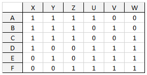
In this example, a so-called acceptable solution 5 is the set of blocks covering all the elements 1 of the given matrix. It is required to choose a feasible solution containing the minimum possible number of blocks, i.e., so-called optimal solution (Figure 01 ).

See Full Size >

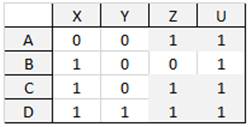
In Figure 01 below, we give a simple example to this problem. The table has the following 5 grids:

α = {A,B,C,D}×{U}; β = {A,C,D}×{Z,U};

γ = {B,C,D}×{X,U}; δ = {C,D}×{X,Z,U};

and ω = {D}×{X,Y,Z,U}

(we selected the elements of the block in a gray background). To cover all the 1’s of the given matrix, it is sufficient to use 3 of these 5 blocks, namely β, γ and ω.

The second example: minimization of DNF

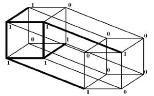
Now, let us give the formulation of the problem of minimizing disjunctive normal forms (DNF). An n-dimensional cube is specified, and each vertex is marked with 0 or 1 elements. An admissible solution is the set of k-dimensional planes of this cube (where the values of k are, generally speaking, different for each plane, not exceeding n), containing only 1’s and covering all elements 1 of the given n-dimensional cube. It is required to choose a feasible solution containing the minimum number of planes. In this case, as in the previous problem, we will additionally require that none of the planes considered be contained in any plane of greater dimension (Figure 02 ).

See Full Size >

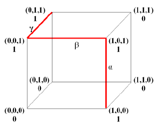
A simple example is shown on Figure 02 . Here n = 3 (that is, we are considering the “ordinary” cube), and there are 3 planes, each of which has a size of 1 (that is, a segment):

α = [(1,0,0),(1,0,1)], β = [(0,0,1),(1,0,1)], and γ = [(0,0,1),(0,1,1)].

For the coverage, it is sufficient to choose 2 of these 3 planes: α and γ.

The third example: traveling salesman problem

Third, let us consider the traveling salesman problem (TSP). It defines a matrix in which the cost of travel from the i-th city to the j-th one is recorded in the cell located at the intersection of the i-th string and the j-th column. It is required to make a route (tour) of the traveling salesman, passing through all cities, starting and ending in the same city; each of the tours and is an acceptable solution. It is required to choose a feasible solution with the lowest possible cost (Figure 03 ).

See Full Size >

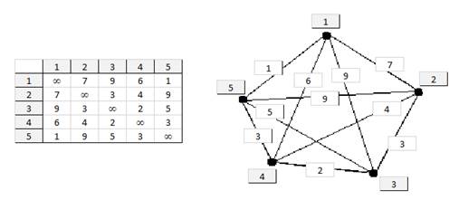
A simple example is shown in Figure 03 , it shows two ways of specifying the same particular case of TSP. For small dimensions, the input data is often represented as a graph. If the cost of travel “there” and “back” for all pairs of cities coincide, then such a graph is conveniently considered not to be oriented; we will consider only such examples. In this case, the matrices are symmetric with respect to the main diagonal, therefore in our example the elements lying below the main diagonal cannot be specified.

Findings

The whole set of admissible solutions in other words is called the state space. Practically for each problem, there is the possibility of an effective auxiliary algorithm designed to obtain some new feasible solution based on the already available one; so the entire state space can be considered a graph. Usually, such graph is undirected. Figures 4 shows possible graphs describing the state spaces for the examples that we already considered: the figure on the left is for the problem of DNF-minimizing, and the figure on the right is for the problem of NFA-minimizing. We believe that in both examples, a new solution can be obtained on the basis of the previous one by deleting or adding exactly one element (the plane or the grid), but we note that other relevant auxiliary algorithms are often used. In both figures, the optimal solutions are highlighted (Figure 04 ).

See Full Size >

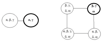
In the given examples, the state spaces are small. However, in real conditions, their size often exponentially (and more) depends on the size of the input data. Therefore, the search for an acceptable admissible solution in such a graph is the most important point in the algorithmization of hard problems. This search corresponds to the construction (explicit or implicit) of a subgraph that is a so-called root tree. And the natural procedure for constructing (sorting out the vertices) of this tree is called backtracking, simple examples of which can be found in most books on artificial intelligence, (Melnikov & Melnikova, 2017; Melnikov & Pivneva, 2016; Melnikov & Melnikova, 2018) etc.

The word “heuristic” has already been mentioned above. There are many different definitions of this concept – and sometimes they even contradict each other, and in some (worse) books, they are unsuccessful. For the word “heuristics”, there is often (“almost correct”) interpretation of “decision-making under uncertainty”. Heuristic algorithms usually do not guarantee an optimal solution; but with an acceptable high probability, they give a solution that is close to optimal. At the same time, their variants are often needed, the so-called anytime-algorithms, i.e., real-time algorithms that have the best (at the moment) solution at each particular moment of the work; the user in real time can view these pseudo-optimal solutions. The sequence of such solutions in the limit usually gives the optimal solution.

Greedy algorithms and their drawbacks

The simplest example of heuristic (but not anytime) algorithms is, apparently, greedy algorithms. A little simplifying the situation, we can say that they consistently build a solution in several steps, at each step, including the “part of the permissible solution”, which at the moment seems to be the most profitable. For example, in problems of minimizing finite automata and disjunctive normal forms, this is a grid (a plane) adding to the current solution the maximum number of new cells in which 1 is written. And in TSP, it is an element of the matrix (from those that can be added to the construction round), which has a minimum cost.

It seems at first glance, that greedy heuristics are very good. However, for each of the problems we are considering, it is easy to come up with examples when this is not so. We have already considered just such examples, for problems of minimizing disjunctive normal forms and nondeterministic finite automata. Moreover, it can be shown that a greedy algorithm can give solutions whose values are arbitrarily greater than optimal ones.

Let us consider two simple examples. Suppose that for the NFA-minimization problem, the table is given as follows (Figure 05 ). At the same time, the greedy heuristics will choose one of two maximum grids, for example, the grid corresponding to the rows A, B and C and the columns X, Y and Z. However, both maximal blocks are not included in the optimal answer: one of such possible optimal answers is 6 “grids-strings”, in which for each letter from A to F, we simply “include all possible 1’s”.

See Full Size >

Figure 06 for the problem of minimizing DNF is sometimes called “hedgehog”. The plane corresponding to the maximum possible k is not included in the optimal answer: in our case, n = 4, k = 2, and such a plane is the only square marked with bold lines (Figure 06 ). The optimal answer is four “fat” segments, not belonging to this square (“the needles”).

See Full Size >

Of course, both these examples are specially chosen so that the so-called “greedy” algorithms work badly here. However, even in the examples we have examined, there are shortcomings of greedy algorithms on small dimensions of the optimization problems we are considering. In real conditions, all the examples are much more complicated than those given here, but from the “small” examples we have chosen very interesting ones. And it is obvious that in the case of large dimensions, these shortcomings should further “spoil life”, that is, give nonoptimal solutions with much greater probabilities, or give solutions that are farther from optimal ones, etc. The way out of this situation is the use of more complicated heuristics.

Conclusion

In the continuation paper, we propose to give a much more detailed description of BBM, and consider other examples: i.e., the examples of the problems of discrete optimization considered here, as well as some others. Also, in the following publications, we want to briefly consider a number of additional heuristics to BBM, which improve (by different parameters) its work. Let us note once again that the software implementation of such heuristics is quite accessible to “advanced” young students. Here are some of the questions that we want to consider further. There are several subroutines for selecting a separating element – how to choose the only one from their answers? For this choice, we apply the so-called “game” heuristics and risk functions. And simultaneously with the last ones for averaging we apply algorithms from one more area of artificial intelligence, i.e., so called genetic self-learning algorithms. Where, as in them, there should be “the desire of the program for self-improvement”? But this is a big separate topic, which we also want to present later.

As the latest scientific publications of authors on this subject, we mention Melnikov & Melnikova (2017), Melnikov & Pivneva (2016), Melnikov (2018), Melnikov (2017).

References

1. Goodman, S., & Stephen, S. (1977). Introduction to the Design and Analysis of Algorithms. NY: McGraw-Hill Computer Science Series.
2. Lipski, W., (2004). Kombinatoryka dla programisto´w. Warszawa, Polish: Wydawnictwa Naukowo-Techniczne.
3. Luger, G. (2008). Artificial Intelligence: Structures and Strategies for Complex Problem Solving. Boston, US: Addison Wesley
4. Melnikov, B. (2017). The complete finite automaton: International Journal of Open Information Technologies, 5(10), 9-17.
5. Melnikov, B. (2018). The star-height of a finite automaton and some related questions: International Journal of Open Information Technologies, 6(7), 1-5.
6. Melnikov, B., & Melnikova, A. (2018). Pseudo-automata for generalized regular expressions: International Journal of Open Information Technologies, 6(1), 1-8.
7. Melnikov, B., & Melnikova, E. (2017). Waterloo-like finite automata and algorithms for their automatic construction: International Journal of Open Information Technologies, 5(12), 8-15.
8. Melnikov, B., & Pivneva, S. (2016). On the multiple-aspect approach to the possible technique for determination of the authors literary style. In Vladimir Sukhomlin, Elena Zubareva & Manfred Shneps-Shneppe (Eds.). The 11th International Scientific-Practical Conference Modern Information Technologies and IT-Education: CEUR Workshop Proceedings. Selected Papers SITITO 2016 (pp. 311-315). Moscow: SITITO.
9. Nonogram (2018). https://en.wikipedia.org/wiki/Nonogram. Last accessed 14 June 2018
10. Pivneva, S., Melnikov, B., & Kuptsov, N. (2016). Infinitely complex sum of classification of non-commuting matrix S-sets. The 1st International Scientific Conference Convergent Cognitive Information Technologies: CEUR Workshop Proceedings. 1. Сер. "Selected Papers of, Convergent 2016" (pp. 56-63).
11. Pola´k, L. (2005). Minimizations of NFA using the universal automaton: International Journal of Foundations of Computer Science, 16(5), 999–1010. Sudoku, http://www.sudoku.com. Last accessed 14 June 2018.
12. Russel, S., & Norvig, P. (2010). Artificial Intelligence: A Modern Approach. NJ: Prentice Hall.
13. Wirth, N. (1979). Algorithms + Data Structures = Programs. NJ: Prentice Hall.