The timely and quickest processing of socio-economic data, their analysis and obtaining new, non-trivial knowledge about the economic condition of an enterprise and the choice of “preferred management” decisions is a key target of economic development. The leadership of industrial enterprises constantly has to decide the question: how should they make decisions to maximize remuneration? The study presents the technology of management decisions at industrial enterprises in the conditions of the digital economy, which allows synthesizing decision support systems. It is shown that using the criteria-based approach to decision-making, it is advisable to formulate a problem statement, select quality criteria, determine controlled parameters, describe disciplining conditions, build a simulation model, make calculations with it and make a decision. Problem statements depending on the availability of information about the set of solutions S and the set of quality criteria F can be of three types: the general decision-making problem, the choice problem, the general optimization problem. The procedure for selecting quality criteria consists of four steps: elimination of ambiguity of goals, harmonization of goals, scaling and ranking. A sequence is proposed that is advisable to use when describing deterministic, random, and indefinite groups of factors. Solutions can be obtained on the basis of identifying the controlled parameters Xi (elements of the solution) and the choice for each particular value Xi = g(xij), as well as the use of search methods for new solutions.
Modern economic development is characterized by such features as innovation, dynamism and globalization. The use of digital information and communication technologies creates a new system of economic relations, called the “digital economy”. The emergence of the digital economy, the accumulation of large amounts of data (big data) requires for the development of methods and means of working with economic information. The timely and quickest processing of socio-economic data, their analysis and obtaining new, non-trivial knowledge about the economic condition of an enterprise and the choice of “preferred management” decisions is a key target of economic development. Constantly we have to solve the question: how should we organize decision-making to maximize remuneration?
A number of papers by domestic and foreign scientists describe various areas of the digital economy:
Enterprise economics: forecasting bankruptcy of enterprises (Evstropov, 2008; Ashmarina, Streltsov, Dorozhkin, Vochozka, & Izmailov, 2016), forecasting sustainable development of enterprises (Bulgakova & Golovaneva, 2012; Orlov, 2011; Bansal, 2005), analysis of labor remuneration and its productivity (Kolesnikova & Kovalerov, 2015; Vaisburd, Simonova, Bogatyreva, Vanina, & Zheleznikova, 2016; Simonova, Bazhutkina, & Berdnikov, 2015), assessment of the financial condition of a business (Pelipenko & Khalafyan 2015), enterprise resource planning (Brazhnikov, Khorina, Minina, Kolyasnikova, & Streltsov, 2016; Lepistö, 2014), product market segmentation (Pogorelova, Yakhneeva, Agafonova, & Prokubovskaya, 2016; Ashmarina, Pogorelova, & Zotova, 2014) and others;
Production processes: modeling the function of production (Matyukhin 2010), modeling of production risks (Potupchik, Pyshnograi, & Tskhay, 2012), production of high-tech products in the industry (Anastasiadi & Silnikov 2013), the use of IT-systems that support business processes at the enterprise (Mesjasz-Lech, 2014) and others.
Problem Statement
Currently, there are quite a number of modern scientific disciplines devoted to the problem of decision making. These include mathematical programming, a game theory, a theory of statistical solutions, a theory of optimal automatic control, economic cybernetics, operations research, system analysis, etc. These disciplines deal with the problem of optimal solutions for different types of control objects and in different conditions of their existence (including industrial enterprises). In this sense, they can be considered as components of a single scientific discipline with the term “decision-making theory” (DMT).
There are three ways to make decisions:
1. A decision is made, prompted by previous life experience (intuition) - an intuitive way.
2. A decision is made on the results of field tests, processed by methods of applied statistics.
3. A decision is made on the results of mathematical modeling.
Decision-making theory at industrial enterprises should answer the following questions:
How should decision-making be organized to maximize profits?
How to act in such conditions when others can impede the implementation of the planned actions?
How to act in such conditions when remuneration can be provided only in the distant future?
Research Questions
To date, the data retrieval procedure and the necessary knowledge extraction from it acquires the greatest relevance.
If earlier the knowledge extraction from information was somewhat creative, then gradually there were templates, which soon grew into special packages, first specialized, and then universal. Systems of algorithms were developed, statistical data processing was developed, hidden patterns came to light (Shepel & Akimov, 2015). Thus, we can talk about the knowledge extraction from a certain set of information that can be formalized. This process is constantly developing and improving, as its methods develop and improve. Data Mining is a collective name used to denote a set of methods for detecting previously unknown, non-trivial, practically useful and accessible interpretations of knowledge necessary for decision-making in various spheres of human activity in data (Dyuk, Flegontov, & Fomina, 2011).
Purpose of the Study
The purpose of the study is to select the technology of management decision-making at industrial enterprises in the digital economy, and to formalize the stages of the technology obtained.
Research Methods
Problem statements
The decision-making procedure begins with the formulation of the problem. Goal setting is a statement of goals (desired results), upcoming actions and the conditions in which they must be performed. We distinguish three different, albeit interrelated, ways in which goals arise:
1. Based on the study of the theory. We study all available environments in order to search for new ideas, theories, methods, materials and devices, and then offer ways to use them at the enterprise.
2. Based on the study of practical needs.
3. We are waiting for specific instructions on the development of new methods for the application of technology and production technology.
The wait method often precludes reasonable planning (due to lack of time) of an action program; when specific instructions, the only way out may be to achieve the goal at any cost. Ultimately, the wait method is the most expensive.
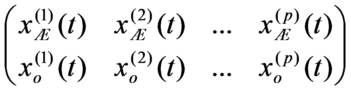
The problem statement based on a study of practical needs can be described as follows. Original statistical data for the analysis are conveniently presented as a matrix.
To preliminarily formulate the problem based on the study of practical needs it is suggested to use the concept of homogeneity or a measure of proximity. In the general case, the concept of homogeneity of the state of objects is defined either by introducing the rule for calculating the distances
Figure 32:
See Full Size > between any pair of objects under study, or by specifying some function
Figure 33:
See Full Size > ,characterizing the degree of proximity of the
i
th and
Figure 34:
See Full Size >th states of objects. If a function is specified
Figure 35:
See Full Size >, then from the point of view of this metric, the states of objects are considered to be homogeneous, belonging to the same class. Obviously, it is necessary to compare
Figure 36:
See Full Size >with some threshold (desired) values
Figure 37:
See Full Size >, determined in each case in their own way. If
Figure 38:
The choice of a metric or a proximity measure is the key point of the study. In each particular case, this choice should be made in its own way, depending on the purposes of the study, the physical and statistical nature of observations of
X
, a priori information about the nature of the probability distribution of
X
.
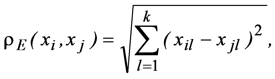
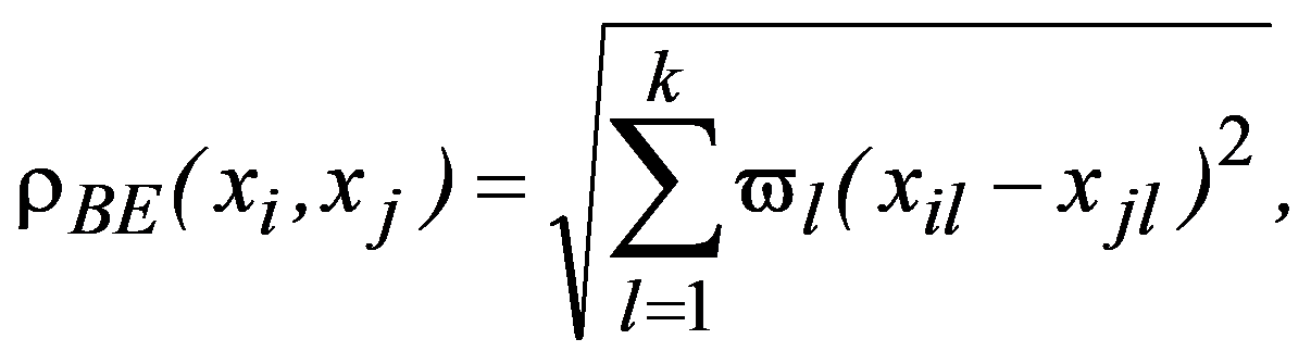
For many management decision-making problems (including for industrial enterprises), it is advisable to use Euclidean space as a metric
Naturally, from a geometric point of view, Euclidean space may be meaningless (from the point of view of a meaningful interpretation), if features are measured in different units. To correct the situation, they resort to rationing each feature by dividing the centered value by the standard deviation and go from the matrix
Х,
to the normalized matrix with the elements:
The classification of general decision problem depending on the availability of information on the set of solutions to
S
and the set of quality criteria
F
is given in the Table
01
:
So, for the preliminary formulation of the problem based on the study of practical needs, it is proposed to use Euclidean space or “weighted” Euclidean space.
Selection of quality criteria
To compare the degree of the goal achievement with the help of the chosen method, they use quality criteria, which are a mathematical expression of the goal (a mathematical model of the goal).
The informal procedure for the selection of quality criteria necessary to substantiate decisions at industrial enterprises is presented. The procedure includes four steps:
1) Eliminate the uncertainty of goals, i.e. formulate and write down all the goals that we pursue under this task;
2) Coordinate the obtained list of goals among themselves and with the goals of the parent body;
3) Select a unit and scale of measurement for each goal (to scale), i.e. with this informal operation, we transit the goals into quality criteria;
4) Rank the quality criteria, i.e. rank the criteria in order of importance.
In drawing up a list of goals, we will be helped by: turning to authority; expert analysis; use of casuistic methods.
Disciplining conditions
In any decision-making there are factors that limit the ability to achieve the goal. They are also called “disciplining conditions”.
Among the disciplining conditions may be deterministic, random and indefinite groups of factors. A procedure is proposed that is advisable to use when describing factors that limit the ability to achieve the goal of any operation:
1. From all the parameters characterizing the planned operation, select a set of disciplining conditions and a set of decision elements.
2. From all disciplining conditions, select deterministic, stochastic and uncertain factors.
3. For random factors, consider the possibility of averaging the parameters of disciplining conditions or averaging performance indicators or introducing statistical restrictions.
The review made it possible to identify eleven different methods identifying the laws of distribution, each of which has its own advantages and disadvantages. However, there are several common features of most or all of the above methods:
All methods require the participation of an expert in the field of statistics;
Most of the methods are difficult to calculate. For example, the widely used Parzen-Rosenblatt method involves calculating the value of the blur parameter, and the task of estimating its optimal value is more complex than the original problem of restoring the distribution density;
All methods (except the method of constructing histograms) imply a procedure for comparing experimental values with a certain theoretical distribution, which, in the case when the proposed distribution laws are numerous, forces the researcher to carry out the identification procedure many times, rejecting by its results only one distribution law, if the hypothesis of compliance is not confirmed;
The method of constructing histograms has very low accuracy, and is more often used only for formulating hypotheses, and not for strictly identifying the distribution law.
In the practice of statistical analysis and modeling, the exact form of the distribution law of the analyzed population is, as a rule, unknown. We have only a sample of the general population of interest (Shepel, 2012). If these are simultaneous observations for a single feature, then the matrix of sample data is:
We are forced to build our conclusions and make decisions based on the calculation of a limited number of sample characteristics. The main selective (empirical) characteristics (Ayvazyan & Mkhitaryan 2001), as a rule, include:
See Full Size >); sample data that fall on the boundaries of intervals, or evenly distributed over two adjacent intervals, or referred only to any one of them are calculated;
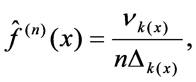
For each interval, the empirical density function
Figure 95:
By the type of histogram, the hypothesis about the model of the distribution law of the analyzed general population (for example, normal, exponential, uniform, etc.) is accepted;
Estimates of unknown parameters of the hypothetical distribution law
Figure 105:
See Full Size >are calculated (for example, for the normal distribution law, the sample mean
Figure 106:
See Full Size > is obtained. There is a need for experimental verification of the hypothesis about the type of the distribution law of the analyzed population, i.e. our goal is to check whether the hypothesis
Figure 109:
See Full Size >expressed does not contradict the existing sample data.
The problem can be solved qualitatively or quantitatively (Shepel, 2012).
4. Divide the indefinite factors into types: a) the probability distribution for the parameters ξ exists in principle but cannot be obtained by the time the decision is made, and b) the probability distribution for the parameters ξ does not exist at all.
For type a), accept the hypothesis about the nature of uncertain factors or try to use adaptive methods.
For type b), choose plausible parameters for uncertain factors or determine the possible range of variation of uncertain parameters or determine the worst strategy for the competitor’s behavior.
Elements of decision-making
Those parameters, the combination of which forms a solution, are called decision elements. The elements of the solution may include various numbers, vectors, functions, physical attributes, etc.
The elements of the solution
X
i
are sets consisting of a finite number of discrete values
х
ij
Figure 110:
See Full Size >
X
i
or continuous values from a certain interval ]
x
i0
,x
in
[.
A solution variant (solution alternative) of a decision is a set of decision elements (controlled parameters), each of which is assigned a specific value from the set of permissible
x
vi
= <
x
1j
,...,x
rk
,...,x
mn
>.
Solutions can be obtained on the basis of:
- Identify the controlled parameters Xi
X
i
(solution elements) and select for each specific value
X
i
= g(x
ij
);
- Use methods for finding new solutions.
Simulation
In the process of making decisions, it seems appropriate to use stimulation models. In simulation, the model-implementing algorithm reproduces the process of system
S
in time and simulates the elementary phenomena that make up the process, while preserving their logical structure and sequence of flow in time.
There could be two types of simulation models: controlled and forecast. Controlled models answer the questions “What will happen if ...?”; “How to achieve the desired?”, And contain three groups of variables: 1) variables characterizing the current state of the object; 2) variables affecting the change of this state and amenable to purposeful selection (control actions); 3) source data and external influences, i.e. external parameters and initial parameters. In forecast models, control is not explicitly highlighted. They answer the question: “What will happen if everything is the same?”
The process of modeling at industrial enterprises is reduced to the implementation of three stages. At the stage of building a model and its formalization, a study of a simulated object is carried out in order to identify the main components of its functioning process. The necessary approximations are determined, and a generalized system model diagram is obtained. This scheme is converted into a machine model at the second stage of modeling by sequential algorithmization and programming of the model. The last third stage of system modeling is reduced to carrying out working calculations on a computer, as well as obtaining and interpreting the results of system modeling.
Decision-making
If a single-criterion problem is solved, then choosing a solution, we naturally prefer one that turns the quality criterion to a maximum (or to a minimum).
In practice, single-criteria problems are rare. Usually, decision-making is characterized by several criteria, which should be turned into a maximum and others into a minimum. A solution that simultaneously satisfies all these requirements is missing. A solution that reverts to a maximum of one kind of criterion, as a rule, does not draw either the maximum or the minimum of others.
When solving multi-criteria decision-making problems (Shepel & Speshilova, 2016; Kitaeva, Speshilova, & Shepel, 2016), a number of specific problems arise that are not computational, but conceptual.
In vector optimization problems there is a contradiction between some of the criteria. This contradiction is usually weak, because otherwise the problem becomes a conflict antagonistic one. By virtue of this, the domain
Figure 111:
See Full Size >of feasible solutions splits into two disjoint parts: the domain of agreement
Figure 112:
Further search for optimal solutions in the domain of compromise can only be carried out on the basis of a certain compromise scheme. The choice of a compromise scheme corresponds to the disclosure of the optimization operator, usually in the form
See Full Size >is some scalar function of the criteria vector
E
.
Thus, the choice of one or another principle of optimality reduces the vector decision-making problem to the equivalent (in the sense of the accepted principle of optimality) scalar decision-making problem.
In those problems in which local criteria have different units of measurement, it is necessary to normalize the criteria, i.e. bring them to a single, preferably dimensionless, scale of measurement.
Usually local criteria have different importance. This should be considered when choosing the optimal solution, giving a well-known preference to more important criteria.
These problems are conceptual in nature, when solving them it is necessary to resort to various kinds of heuristic procedures in which experts play a significant role.
The most suitable for use by the decision maker (DM) is the method of successive concessions. Suppose that the criteria
f
1,
f
2,
..., f
n
are arranged in decreasing order of importance. First, we are looking for a solution that turns the first (most important) indicator
Figure 119:
See Full Size >into a maximum. Then we assign, based on practical considerations, some “concession”
Figure 120:
See Full Size >, which we agree to make in order to maximize the second indicator
f
2. Next, again assign a “concession” to
f
2, at the cost of which you can maximize
f
3; and so on. Such a way to build a compromise solution is good because here you can see immediately the price of “concession” in one criterion gained in another and what is the magnitude of this gain.
Findings
It has been established that the intuitive way of decision-making gives a big mistake, field tests are not always possible to organize. It is most acceptable to make decisions using mathematical modeling.
To preliminarily formulate the problem on the basis of the study of practical needs, it is proposed to use Euclidean space or “weighted” Euclidean space.
An informal procedure is proposed for selecting the quality criteria necessary for substantiating decisions at industrial enterprises.
A procedure is proposed that is advisable to use when describing the factors that limit the ability to achieve the goal.
When making decisions, it seems appropriate to use stimulation models.
The most suitable for use is the method of successive assignments.
Thus, the study describes a rational decision-making procedure for decision-makers of industrial enterprises consisting of preliminary formulation of the problem, selection of optimality criteria, formulation of disciplining conditions, drawing up a list of alternatives, building a simulation model and decision-making.
Conclusion
In conclusion, over the past two decades, information technologies in manufacturing and business have gone beyond conventional computerization and automation - they have become the basis for the effective use of financial management and marketing, successful management of enterprise resources and customer relationships. Moreover, information technologies gave business access to serious potential accumulated in scientific fields: statistical analysis and numerical modeling, theories of complex systems and neural networks (Breeders, Speshilova, & Taspaev, 2015; Speshilova, 2010). To date, there are a lot of different information products that can carry out a wide variety of calculations. The input data can be quite easily processed using applied statistical packets, however, in practice, in the process of analyzing incoming information and its statistical processing, one may encounter, for example, that the type of the distribution law (which an unknown analyzed data array would obey to) is not determined. This leads to an incorrect application of data processing, and therefore to an incorrect conclusion that, in consequence, will lead to a high error of solutions made. Therefore, a properly organized technology for extracting knowledge from economic databases contributes to effective management decision-making procedures, which is far from important for industrial enterprises operating in the digital economy.
References
Anastasiadi, G.P., & Silnikov, M.V. (2013). Quality management in the production of high-tech industrial products. The legal field of the modern economy, 10, 92-100.
Ashmarina, S. I., Pogorelova, E. V., & Zotova, A. S. (2014). Improving marketing information system of an industrial enterprise as the most important element of change management system. Actual problems of economics, 11 (161), 348-354.
Ashmarina, S.I., Streltsov, A.V., Dorozhkin, E.M., Vochozka, M., & Izmailov, A.M. (2016). Organizational and economic directions of competitive recovery of Russian pharmaceutical enterprises. Mathematics Education, 11 (7), 2581-2591.
Ayvazyan, V.S., & Mkhitaryan, S.A. (2001). Applied statistics. Basics of econometrics: Textbook for Institutes of Higher Education: in 2 Vol. Vol.1: Probability theory and applied statistics. 2nd edition, revised. Moscow: IuNITI-DANA
Bansal, P. (2005). Evolving sustainably: A longitudinal study of corporate sustainable development. Strategic. Management Journal, 26(3), 197-218.
Brazhnikov, M.A., Khorina, I.V., Minina, Y.I., Kolyasnikova, L.V., & Streltsov, A.V. (2016). System development of estimated figures of volume production plan. International Journal of Environmental and Science Education, 11 (14), 6876-6888.
Breeders, N.D., Speshilova, N.V., & Taspaev, S.S. (2015). The use of neural network technologies in predicting the efficiency of grain production. News of Orenburg State Agrarian University, 1 (51), 216-219.
Bulgakova, I.N., & Golovaneva, V.V. (2012). Improving methods for predicting sustainable development of an enterprise based on logit analysis. Modern economy: problems and solutions, 1 (25), 146-150.
Dyuk, V.A., Flegontov, A.V., & Fomina, I.K. (2011). Application of data mining technologies in the natural sciences, technical and humanitarian areas. News of Herzen Russian State Pedagogical University, 138, 77-84.
Evstropov, M.V. (2008). Evaluation of the possibility of forecasting bankruptcy of enterprises in Russia. Bulletin of the Orenburg State University, 4 (85), 25-32.
Kitaeva, M. V., Speshilova, N. V., & Shepel, V. N. (2016). Mathematical models of multi-criteria optimization of subsystems of higher educational institutions. International Review of Management and Marketing, 6(S5), 249-254.
Kolesnikova, S.V., & Kovalerov, N.V. (2015). The use of special econometric models for the analysis of wages. Regional economy: theory and practice, 15 (390), 48-55.
Lepistö, L. (2014). Taking information technology seriously: on the legitimating discourses of enterprise resource planning system adoption. Journal of Management Control, 25, 193-219.
Matyukhin, V.V. (2010). Model of production function based on the law of diminishing productivity. Bulletin of Kamchatka State Technical University, 13, 30-34.
Mesjasz-Lech, A. (2014). The use of IT systems supporting the realization of business processes in enterprises and supply chains in Poland. Polish Journal of Management Studies, 10(2), 95.
Orlov, A.I. (2011). Sustainable economic and mathematical methods and models. Development and development of sustainable economic and mathematical methods and models for the modernization of enterprise management. Saarbrücken, Germany: LAP (LAMBERT Academic Publishing
Pelipenko, E.Yu., & Khalafyan, A.A. (2015). Information system of decision-making support in the field of assessing the financial status of small and medium-sized businesses. Polythematic network electronic scientific journal of the Kuban State Agrarian University (Scientific journal of KubGAU, 4 (108), 872-890.
Pogorelova, E.V., Yakhneeva, I.V., Agafonova, A.N., & Prokubovskaya, A.O. (2016). Marketing mix for e-commerce. International. Journal of Environmental and Science Education, 11 (14), 6744-6759.
Potupchik, A.V., Pyshnograi, G.V., & Tskhay, A.A. (2012). Risk modeling for output. Bulletin of Altai Academy of Economics and Law, 1, 87-90.
Shepel, V.N. (2012). The procedure for constructing a sample analogue of the density function. OGU Bulletin, 2 (138), 320-322.
Shepel, V.N., & Akimov, S.S. (2015). Problems of knowledge extraction. In Materials of the All-Russian scientific and methodical conference “University complex as a regional center of education, science and culture” (pp.1562-1565), Orenburg: Publishing Center OGU.
Simonova, M.V., Bazhutkina, L. P., & Berdnikov, V. A. (2015). Approaches to the system salary increase in the region on the ground of labor production growth. Review of European Studies, 7 (2) 2015, 58-65.
Speshilova, N.V. (2010). Information technologies in accounting. In Karakulev V.V. (Ed.), Proceedings of the international scientific-practical conference “The state, prospects of economic and technological development and environmentally safe production in the agricultural sector” Part II (pp.30-36). Orenburg: Publishing Center OGAU.
Vaisburd, V.A., Simonova, M.V., Bogatyreva, I.V., Vanina, E.G., & Zheleznikova, E.P. (2016). Productivity of labour and salaries in Russia: problems and solutions. International Journal of Economics and Financial Issues, 6 (S5), 157-165.
Business, business ethics, social responsibility, innovation, ethical issues, scientific developments, technological developments
Cite this article as:
Shepel,
V.,
Speshilova,
N.,
&
Kitaeva,
M.
(2019). Technology Of Management Decision-Making At Industrial Enterprises In The Digital Economy. In
V.
Mantulenko
(Ed.),
Global Challenges and Prospects of the Modern Economic Development, vol 57. European Proceedings of Social and Behavioural Sciences (pp. 1520-1531).
Future Academy. https://doi.org/10.15405/epsbs.2019.03.155
We use cookies or similar technologies to access personal data, including page visits and your IP address.
We use this information about you, your devices and your online interactions with us to provide, analyse and improve our services.
This may include personalising content or advertising for you. You can find out more in our
privacy policy and
cookie policy and
manage the choices available to you at any time by going to ‘Privacy settings’ at the bottom of any page.
Manage My Preferences
You have control over your personal data. For more detailed information about your personal data, please see our
Privacy Policy and Cookie Policy.
These cookies are essential in order to enable you to move around the site and use its features, such as accessing secure areas of the site.
Without these cookies, services you have asked for cannot be provided.
Third-party advertising and social media cookies are used to
(1) deliver advertisements more relevant to you and your interests;
(2) limit the number of times you see an advertisement;
(3) help measure the effectiveness of the advertising campaign; and
(4) understand people’s behavior after they view an advertisement.
They remember that you have visited a site and quite often they will be linked to site functionality provided by the other organization.
This may impact the content and messages you see on other websites you visit.