The Time Horizon Of Asset Price Movements To Predict Financial Crises

Stock and Gold Price Fluctuations

As stated earlier, the extreme price deviation of an asset from its fundamental value makes price bubbles. These bubbles burst and send ripples in the entire economy and make a financial crisis. Stock markets are one of the most busy asset markets across the globe. So much of stock volume is traded every day and this makes it one of the most volatile markets as well. (BATES, 1991) states that in stock markets, bubbles are most of the time rational. By rational bubbles, author means that development in stock markets is almost visible to the investors who know when stocks are overpriced. Overpricing means at some future point prices will have to come down and this is very easily spotted in share markets. Author also indicates that even though the bubble is rational, it bursts when prices come down. The same is discussed by (Chen, Hong, & Stein, 2001), who further this in their study and state that the volatility in stock markets is linked with the price fall. Authors say that in stock markets, it is the price melt-down rather than price build up that injects volatility in the market. It is also observed that any information in form of good news or bad news enters in the market, it increases risk premium which investors do not like and thus the price fall happens. Since stock markets are very busy and tons of trade happens daily, this means that stock markets are more volatile as more business is done there. Volatility means stock markets are not stable. (Eraker, 2004) also talks about volatility in share markets and states that this volatility increases over time. With a longer time horizon, volatility is observed to have increased with the change in share prices. Author also says that this happens due to increased uncertainty about share prices. This is a very interesting find because it incorporates factor of time along with price bubbles. With such bubbles present in stock markets, it can be said that many crashes must happen in share markets but this is not so. (Gilchrist, Himmelberg, & Huberman, 2005) share a very interesting trend in stock markets and state that actually the price hike or the bubble is normalized in share markets with the issuance of new shares. When the share prices rise, new issues are released causing the overall price rise to settle down a bit. Authors also say that dispersion in investors’ beliefs is also a reason why price bubbles are formed but do not end up as harmful. As for the Gold markets, (Lili & Chengmei, 2013) say that gold prices are negatively affected by macroeconomic factors as well as financial market indices. So, when an economy is facing hard times gold prices rise and vice versa. As for the prediction of gold prices, (Pierdzioch, Risse, & Rohloff, 2014) state that gold prices are linked to business cycles. According to the study, the ups and downs in the gold prices are predictable by understanding the trends in gold markets.

The factor of Time in Asset markets

In Asset markets, all the transactions are time bound yet the data on role of time in asset markets in least available. Even though multiple studies indirectly include time, but the direct effects of time are still not well known. (Friedman, Laibson, & Minsky, 1989) talk about markets crashes and price bubbles with respect to time and say that once a market crash happens, it indicates a larger price bubble over a longer time period. Such a bubble burst happens over long time horizon. Authors argue that this happens due to more information adds up in long run which can be used as a tool to predict price bubble formation and subsequent bust. It can be ad that time affects assets by affecting some market variables. This is presented in the study by (Ball, Cecchetti, & Gordon, 1990) who say that actually it is the uncertainty caused by inflation that affects markets. And this affect intensifies in the longer time periods than short time periods. Which means that in short time horizons, uncertainty does not unleash its severity to the fullest and it can only be observed in the long run. (Blanchet-Scalliet et al., 2005) also link uncertainty with market risk and timing risk and state that when a time horizon is unknown, i.e. the time of the occurrence of an event is unknown, market risk increases. Thus time horizon is important in understanding the behaviour of market to predict any negative financial happenings. In a very interesting study (Cecchetti, Lam, & Mark, 1990) state that asset prices revert to their mean values over time. But how much time does it take? They say that this cannot be seen in just five to ten years of time period as asset prices fluctuate and go up and down. So to go back to their mean, takes probably a longer time period. This study leaves with inference that there exists times, where asset price fluctuations can be captured or predicted beforehand. If such a time can be captured it can help avoid any potential crisis from happening.

Another interesting aspect in this regard is explored by (Gordon , 1998) and (Henkel et al., 2011), they talk about time in markets with respect to recession and expansion cycles. Author says that markets which experience fast business or more expansion cycles, the prices decline there. And in such markets, it becomes rather difficult to predict any future crises. Author also takes the research in the dimension of business cycles and state that among these is that time horizon which can lead to predicting and preventing financial crises in economy in general. An economy comprises of many variables an assets and each have their own effects on it. (Goodhart & Hofmann, 2000) relate assets with inflation and state that a shorter time horizon of two years in not enough to study the relationship of house prices with inflation. The full impact of these can be studied over a longer time horizons which can lead to other interesting insights.

Markets operate with information. This information can be of any sort and timing of this information and its impact is very important. This area is explored by (Ehrmann & Fratzscher, 2005) who say that an unexpected information in the market lasts longer. Normally, information is linked with short time horizon as it is incorporated in asset prices there and then. But an unexpected information remains in the market for longer and it remains there and can be detected over long time horizons.

Razen, Huber, & Kirchler, (2017) explain the working of asset markets with respect to the relative lives of the assets. They say that asset markets where trading horizons are longer and assets have longer lives like shares etc., these markets are more prone to price bubble formation. This study shows that not all assets cause financial cries, rather more tradable assets are more prone to such attacks and only in a longer time horizon is it possible to attacks and only in a longer time horizon is it possible to see a possibility of bubble formation. (Noussair, 2017) furthers the life of assets in his study and states that those assets with linger lives see a price fall over longer time horizons. This characteristic makes it possible to predict any dangerous price formation.

The research on importance of time in asset markets suggests the important things. First, information is the most important factor related to time. It is the degree of information seriousness that prevails over longer time horizons and changes investors’ beliefs. Second, assets have their lives too. The longer the life an asset has, the more chances are there to predict the future events in these markets.

Asset price Bust Identification

The main focus of this study is to identify asset price busts in asset markets with respect to time; this study uses the asset price indicator developed by (Gerdesmeier et al., 2010). This indicator will serve as dependent variable in this study to check the cause and impact relationship of asset prices with macroeconomic variables. The composite indicator ΔC includes share prices and gold prices, presented mathematically as;

ΔC = ϕ1ΔShare Prices_t + ϕ2Δ Gold Prices_t

Where, ΔC indicates fluctuation in asset prices. Every time a bust occurs, ΔC falls below a pre-set value. This pre-set value is this case is the peak value of asset prices in the given time period. Asset price bust will occur when ΔC drops or becomes equal to a pre-set threshold in the said time period compared to its highest value in the same time period (Gerdesmeier et al., 2010), it is represented mathematically as;

D t=1 iff ΔC^t+l ≤ (Mean of ΔC - λσ ΔC) Where t is from 1 to t+l

D will be equal to 1 whenever ΔC will drop from its mean minus standard deviation of ΔC from time 1 to t+l. where λ represents a constant, and for this study, it is normalized to 1. This indicates the current price bust. To predict an asset price bust ahead of time, this study follows (Berg & Pattillo, 1999), who created a dummy variable C to indicate a price bust head of time based on current market scenario. The dummy variable C is constructed as represented mathematically as;

C t= 1, Iff Σ D^t+g > 0; where g=1 to i

Note that, C depend on dummy variable D, i.e. if in a certain time period if summation of D is greater than zero, it indicates presence of a price bust in future. In case of present study, four months, six months, twenty four months and sixty months are used as the testing time horizons. All necessary calculations are done in these time horizons. Now, if Dummy variable C signals for a price bust in future, but dummy variable D does not indicate so, then this will be counted as false signal. But not necessarily a wrong signal due to the fact that asset prices are affected even by the investors’ behaviour. Therefore, the notion of wrong signals is not being used in the present study.

After the predictions based on asset prices are made, next come the affect the economy put on asset prices. To understand this cause and effect relationship, this study uses binary regression model, Logit (logritham + Unit) regression analysis. Logit regression is used to predictive analysis and generates results as probability of the occurrence of an event. The reason to use logit regression is to check out the possibility of occurrence of price bust in the presence of various independent variables in the tested time period. The general form of logit regression model is as follows;

Logit (C_ik = 1) = βo + βit . X_ik + ε_ik

Where, X_it represent independent variables, βik represent respective coefficients, and ε_ik represents the error term. Fundamental variables are used as growth rates. Logit regression is first applied to individual variables in all four time horizons to scoop out the significant variables. Then multi-variate logit regression is applied on the significant variables in all four time horizons to check the collective cause and effect of independent variables on the dependent variable.

Occurrence of Bust

To indicate the bust occurrence of asset prices, present study developed a bust indicator which is shown as a dummy variable D. This dummy variable is then studied in different time horizons which in this study are 6 months, 1 year (12 months), 2 (24 months) years and 5 years (60 months). The dummy variable D shows the occurrence of asset price bust in the selected time horizons with respect to the maximum value of assets in the same time period. Table 01 shows four dummy variables for four different time horizons.

Table 01 shows the number of bust occurrences in different time horizons in asset markets. From the table, it is clear that asset markets were facing almost constant number of bust occurrences for almost all the years except for 2004, 2005 and 2009 when tested for 6 months- time span. While in one year time horizon, asset prices faced the extreme fluctuations in the year 2011 followed by 2008 and 2006. While in the 2 year time span, year 2009 shows the extreme fluctuations proceeded by 2008 and followed by 2012. While in the five year time horizon four consecutive years show extreme price fluctuations which means, in these four years, asset markets in Pakistan were constantly facing price bubbles formation and busts. The graphical representation of the bust dummy variable is given below.

See Full Size >

See Full Size >

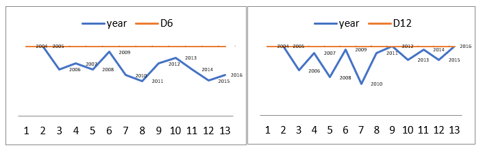
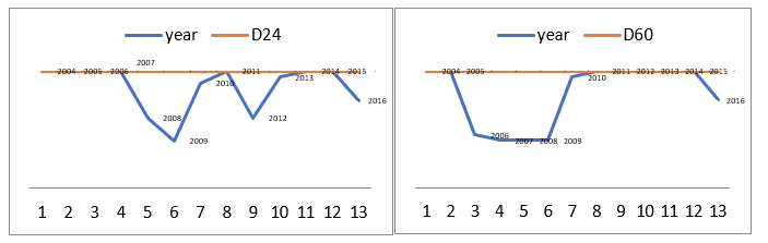
To predict the price busts ahead of time, i.e. in the future, the composite indicator C is tested in the proposed time horizons to check if any price busts can be predicted ahead of time effectively. Table given below presents the comparison.

When compared with Table 01 , Table 02 shows only accurate results produced by C60. This indicates that, whatever bubble busts were predicted by C60 resulted in exactly the same in reality while the other predictions are mostly false alarms which could be due to the presence of other forces in asset markets which lead to normalization of asset prices in real time. But it is too early to come up to a conclusion merely based on asset prices. It is known that asset price do not act alone. Any development is them depends on the economy as well. This suggests that at some previous stage, markets might not be showing promising results, but later on, due to the development in economic variables, asset prices turn out to be more stable and less fluctuating. Graphical representation of these results is given below.

See Full Size >

See Full Size >

See Full Size >

See Full Size >

To know more, Logit regression analysis is applied to understand the behaviour of asset prices in the presence of macroeconomic variables.

Logit Regression analysis

In order to check how much are asset prices affected by the factors in the economy, univariate and multivatriate logit regression is applied to the data. Since this study’s main focus is on the effect of time horizon, therefore the logit regression test is performed on all four time periods. The results are shown in the comparative table 03 .

The tables represent the uni variate logit regression analysis of the selected variables. The tables contain z stat, and their corresponding p-values. The reason p values are included is to help out in the comparison of all four time horizons. The McFadden R-squared values tell the probability of a bust occurrence due to the said variables. In 6 months (Table C6), there are only two variables that affect asset prices significantly, Real-GDP (GDPR) and Monetary aggregate (M2). Even though, money does not show a strong effect on asset prices but it still leaves its impact compared to other variables in the same time period. In 6 months’ horizon, McFadden R-squared values for real-GDP and Money are greater than other variables and show greater likelihood of predicting crisis compared to other variables.

In 12 months’ time span (tables C12), the relatively significant variables are real-GDP, the Credit to the private-sector (CPS), the interest-rate for long term (LTIR) with a negative value, the interest rate for short term (STIR). The McFadden R-squared values for GDPR, CPS, LTIR and STIR are better than other variables and show greater fit and more likelihood of crisis prediction than other variables in the same time period.

In 24 months’ time span (Table C24), the variables that show significant behaviour are GDP-deflator (GDPD) and relatively significant variables are the stable interest rate (LTIR), M2 and the real exchange rate (REER) with negative values. McFadden R-squared values of GDP-deflator and long-term-interest-rate are more than other variables and show that their probability of predicting an upcoming crisis in the asset markets is more than other variables.

In the 60 months’ time span which is 5 years’ time period, the significant variable are the GDP-deflator, the consumer-price-index (CPI), the Credit to the private-sector (CPS), nominal-effective-exchange-rate (NEER) and Short interest rate (STIR). Whereas relatively considerable impact is exerted by the Real-GDP (GDPR), the stable rate of interest (LTIR) and the real exchange rate (REER). The McFadden R-squared values of GDP-deflator, Consumer-Price-Index, Credit-to-Private-Sector, REER, REER and STIR show that the odds of predicting the crisis in the long run of these variables are stronger.

The results show that Real-gross-domestic-product (GDPR) does not impact asset price movement much in the long run. But in longer time period, greater than five years, Real GDP might be an effective tool to adjust asset prices. GDP-deflator (GDPD) it grows stronger and leaves greater impact on asset price misalignments in the long run. Therefore, it can be said that inflation affects asset prices more in longer time horizon compared to shorter time horizons. Consumer-price-index (CPI) also leaves much impact on asset prices in the longer time periods as compared to shorter time periods. The other variables that grow stronger in affecting asset prices in the bigger time horizon are Credit-to-the-private-sector (CPS), Nominal-exchange-rate (REER) and the interest rate of the short term (STIR). The Stable interest rate (LTIR) and real-exchange-rate (REER) remain in the mild category and may cause asset price fluctuations to some extent. Money supply (M2) shows significant impact only in the shorter time horizon but remains ineffective in the long run. This can be due to strict monetary policy as increased money supply affects the economy adversely.

To understand the collective contribution of significant variables in all the time periods, multi-variate logit regression is applied. The results are shown in the tabular form below.

In 6 months’ time period, only two variables showed significance, Real gross domestic product (GDPR) and M2. When testes together, it is seen that money supply grows relatively less affective with GDPR but still leaves a considerable impact in bubble bust. The McFadden R-squared values rather small with almost 6 present probability of predicting an asset price bubble but this should not be neglected as in the very short run, with just two economic variables, a mere 6 present probability can be strengthened in the presence of other economic factors.

When the time horizon is extended to 12 months, the multivariate logit regression shows that with other variables, Real GDP and short term interest rate show more significant impact on asset price movements. The credit to the private sector and the stable interest rate also show somewhat significance. The McFadden R-squared value shows almost double the likelihood of predicting an upcoming price bubble bust in 12 months’ time span. This shows that as the time horizon widens, so are the economic variables ability to predict financial crisis caused by asset prices. In the 24 month time horizon, the multivariate logit regression analysis shows that the implicit price deflator for GDP (GDPD), the short term interest rate, the stable interest rate and real exchange rate show significance towards predicting a crisis caused by unfavourable asset price movement. The impact of short term interest rate, long term interest rate and real effective exchange rate increases on predicting crisis. The McFadden R-squared value indicates that possibility of crisis prediction with this set of variables increase in a two-year time period almost up to 20 present as compared to one year time span. Finally, the five year or sixty month multivariate logit regression results show that when tested as a group, credit to private sector becomes more significant followed by GDP deflator and short term interest rate. The McFadden R-squared increases to a hundred percent compared to 2 year time horizon.

Two interesting inferences can be drawn from these results. First, in short time horizon, the variables are not mature enough and individually or in a group, they might generate results inconsistent with the ongoing economic conditions. Also, short time horizon cannot be used as an appropriate time period to draw any conclusions. Secondly, as the time horizon expands, macroeconomic variables get mature and take in more information. Based on the overall market scenario and economic conditions, asset price fluctuations can show a pattern of bubble formation and bubble burst. This implies that the likelihood of predicting a financial crisis caused by asset price misalignments increases in the long run.

References

- Ball, L., Cecchetti, S. G., & Gordon, R. J. (1990). Inflation and Uncertainty at Short and Long Horizons. Brookings Papers on Economic Activity, 1990(1), 215. https://doi.org/10.2307/2534528
- BATES, D. S. (1991). The Crash of ʼ87: Was It Expected? The Evidence from Options Markets. The Journal of Finance, 46(3), 1009–1044. https://doi.org/10.1111/j.1540-6261.1991.tb03775.x
- Batool, Z. (2016). ROLE OF MONEY AND CREDIT IN ASSET PRICE MOVEMENTS: A CASE STUDY OF PAKISTAN. International Journal of Innovative Knowledge Concepts, 4(7). Retrieved from http://www.ijikc.co.in/sites/ijikc/index.php/ijikc/article/view/225
- Berg, A., & Pattillo, C. (1999). Predicting Currency Crises: The Indicators Approach and an Alternative. Journal of International Money and Finance, 18(4), 561–586. https://doi.org/10.1016/S0261-5606(99)00024-8
- Blanchet-Scalliet, C., El Karoui, N., & Martellini, L. (2005). Dynamic asset pricing theory with uncertain time-horizon. Journal of Economic Dynamics and Control, 29(10), 1737–1764. https://doi.org/10.1016/j.jedc.2004.10.002
- Cecchetti, S. G., Lam, P.-S., & Mark, N. C. (1990). Mean Reversion in Equilibrium Asset Prices. The American Economic Review, 80(3), 398–418. Retrieved from http://links.jstor.org/sici?sici=0002-8282%28199006%2980%3A3%3C398%3AMRIEAP%3E2.0.CO%3B2-A
- Chen, J., Hong, H., & Stein, J. C. (2001). Forecasting crashes: trading volume, past returns, and conditional skewness in stock prices. Journal of Financial Economics, 61(3), 345–381. https://doi.org/10.1016/S0304-405X(01)00066-6
- Ehrmann, M., & Fratzscher, M. (2005). Exchange rates and fundamentals: new evidence from real-time data. Journal of International Money and Finance, 24(2), 317–341. https://doi.org/10.1016/j.jimonfin.2004.12.010
- Eraker, B. (2004). Do Stock Prices and Volatility Jump? Reconciling Evidence from Spot and Option Prices. The Journal of Finance, 59(3), 1367–1403. https://doi.org/10.1111/j.1540-6261.2004.00666.x
- Friedman, B. M., Laibson, D. I., & Minsky, H. P. (1989). Economic Implications of Extraordinary Movements in Stock Prices. Brookings Papers on Economic Activity, 1989(2), 137. https://doi.org/10.2307/2534463
- Gerdesmeier, D., Reimers, H.-E., & Roffia, B. (2010). Asset Price Misalignments and the Role of Money and Credit*. International Finance, 13(3), 377–407. https://doi.org/10.1111/j.1468-2362.2010.01272.x
- Gilchrist, S., Himmelberg, C. P., & Huberman, G. (2005). Do stock price bubbles influence corporate investment? Journal of Monetary Economics, 52(4 SPEC. ISS.), 805–827. https://doi.org/10.1016/j.jmoneco.2005.03.003
- Goodhart, C., & Hofmann, B. (2000). Do Asset Prices Help to Predict Consumer Price Inflation? The Manchester School, 68(s1), 122–140. https://doi.org/10.1111/1467-9957.68.s1.7
- Gordon, R. J., & Gordon, R. J. (1998). Foundations of the Goldilocks economy: supply shocks and the TimeVarying NAIRU. BROOKING PAPERS ON ECONOMIC ACTIVITY, 297--346. Retrieved from http://citeseerx.ist.psu.edu/viewdoc/summary?doi=10.1.1.604.9819
- Henkel, S. J., Martin, J. S., & Nardari, F. (2011). Time-varying short-horizon predictability☆. Journal of Financial Economics, 99(3), 560–580. https://doi.org/10.1016/j.jfineco.2010.09.008
- Komarek, L., & Kubicová, I. (2011). The Classification and Identification of Asset Price Bubbles. Czech Journal of Economics and Finance (Finance a Uver), 61(1), 34–48. Retrieved from https://ideas.repec.org/a/fau/fauart/v61y2011i1p34-48.html
- Lili, L., & Chengmei, D. (2013). Research of the Influence of Macro-Economic Factors on the Price of Gold. Procedia Computer Science, 17, 737–743. https://doi.org/10.1016/j.procs.2013.05.095
- Loayza, N. V., & Rancière, R. (2006). Financial Development, Financial Fragility, and Growth. Journal of Money, Credit, and Banking, 38(4), 1051–1076. https://doi.org/10.2307/3838993
- Noussair, C. N. (2017). The Discovery of Bubbles and Crashes in Experimental Asset Markets and the Contribution of Vernon Smith to Experimental Finance. Southern Economic Journal, 83(3), 644–648. https://doi.org/10.1002/soej.12195
- Pierdzioch, C., Risse, M., & Rohloff, S. (2014). The international business cycle and gold-price fluctuations. Quarterly Review of Economics and Finance, 54(2), 292–305. https://doi.org/10.1016/j.qref.2014.01.002
- Queiroz, T. B. de, Medeiros, O. R. de, & Neto, J. C. da C. O. (2011). Evidence of speculative bubbles on the BOVESPA: an application of the Kalman filter. Brazilian Review of Finance, 9(2), 257–275. Retrieved from https://ideas.repec.org/a/brf/journl/v9y2011i2p257-275.html
- Razen, M., Huber, J., & Kirchler, M. (2017). Cash inflow and trading horizon in asset markets. European Economic Review, 92, 359–384. https://doi.org/10.1016/j.euroecorev.2016.11.010
- Sarno, L., & Taylora, M. P. (1999). Moral hazard, asset price bubbles, capital flows, and the East Asian crisis: Journal of International Money and Finance, 18(4), 637–657. https://doi.org/10.1016/S0261-5606(99)00018-2l
Copyright information
This work is licensed under a Creative Commons Attribution-NonCommercial-NoDerivatives 4.0 International License.
About this article
Publication Date
01 May 2018
Article Doi
eBook ISBN
978-1-80296-039-6
Publisher
Future Academy
Volume
40
Print ISBN (optional)
-
Edition Number
1st Edition
Pages
1-1231
Subjects
Business, innovation, sustainability, environment, green business, environmental issues
Cite this article as:
Batool, Z. (2018). The Time Horizon Of Asset Price Movements To Predict Financial Crises. In M. Imran Qureshi (Ed.), Technology & Society: A Multidisciplinary Pathway for Sustainable Development, vol 40. European Proceedings of Social and Behavioural Sciences (pp. 895-909). Future Academy. https://doi.org/10.15405/epsbs.2018.05.73