Analysis of Operating Engineered Products

Abstract

The work describes the main stages of the life cycle relating to engineering products, including design, manufacture, operation and product disposal. The work proves that the stage during which a product is used is decisive in the market economy, as the customer makes a decision as to the reasonability of the product purchase. A binary formula is proposed for determining the ongoing reduced costs of using a product. The concept of economically optimal product service life is introduced. We propose formulae for calculating economically reasonable service life and ongoing per-unit operating costs. The problem of replacing old products with new ones is analyzed with a focus on minimizing operating costs. The formulae have been derived for determining the point of time for the cost-effective replacement of old products. The limits and ranges are established within which the consumer has the benefit of products replacement. The results can be used as basis data for designing and manufacturing engineering products.

Keywords: Operational propertiespriceoptimizationcostsservice life

Introduction

Industrial goods can be categorized into manufactured and bulky products due to units used to measure and calculate their quantity: manufactured items are determined in pieces, while bulky products are in tons, cubic meters, liters, etc. In machine building, an article of manufacture is understood not only as a component, subassembly or machine, but also as an aggregated unit as a ship and space vehicle. This type of categorization is featured by their usage: products are subordinate to articles of manufacture, often being semi-finished products used for the manufacture of the latter. Products are consumed and articles of manufacture are used for service; besides, consuming products is a one-time process while articles of manufacture are in use for a certain period of time, specifying their service life.

Currently, the concept of the product life cycle (PLC) is widely used to describe manufactured products, including such stages as product development, its operation and disposal. Thus, developing a product starts with an idea in the form of a design concept being further embodied in a set of design documentation. In the process of designing, the first problem to be solved is an optimal design that meets specific criteria and aimed at optimization based on the requirements of production and product usage. At the stage of product development, material and human resources are involved; as a result, the designed product is launched into production in series of the predetermined volumes. Then this gives rise to the second problem associated with optimization usually focused on reducing production costs.

After the product is brought to market, there is a stage of its usage. At the same time, the third optimization problem is driven by consumer needs and interests, implying minimal operating and maintenance costs and optimal service life, at the end of which the product is subject to disposal. (Kozlovsky, 2003).

The formulated problems for optimizing the product life cycles are not equal but closely connected. In most cases of product-market environments, there exists the so-called "dictatorship of the consumer", because consumers decide whether to buy or not one or another product with respect to their needs and available financing. But "dictatorship of the manufacturer" is possible as well, especially in a monopoly market with no choice for the consumer on the market. This is a rare case for those countries that have adopted their anti-monopoly legislations. The third optimization problem within the stage of product operation is main and decisive, the remaining tasks are subordinate.

Between a consumer and manufacturer there is, as a rule, a seller, having his share from buying and selling contracts. The seller’s role in the product life cycle is aptly described by Henry Ford, calling trade the most legitimate way of theft. However, for the consumer, the seller and manufacturer roll into one that determines a product price on the market. Therefore, they should be considered together in solving the third problem related to optimization.

Methods

During the stage while the product is in operation, on the one hand, the consumer gains from the use of this product, on the other hand, he has operational expenditures, which can be divided into initial costs and current expenses (Amelkin, Loginova, & Prokopiev, 2006). The initial costs include the cost of the product purchase, cost of its installation and commissioning. They play the same role as capital investments at the stage of production. Current expenses are dependent on the purpose and design of the product and may include the cost of electricity, fuel, maintenance, spare parts and so on. They are analogous to production costs within the production process.

Thus, for calculating expenditures to operate and maintain the product in use, it is possible to apply a formula of annual reduced costs (Velikanov, 1990):

where C is the operating costs, rub/year; K is the initial capital investments associated with purchasing the product; E is the norm rate of return on capital investments (E ≈ 0.12 ÷ 0.15).

We have two comments on Formula (1). Firstly, in economic calculations when this formula is not supposed to be optimized, value E is understood as a part of the initial capital investments attributable to a certain period of the product use, usually a calendar year, so rate E has a dimension of 1 / year. Second, there is a wide range of products being developed and modernized in a constant way. Apart from design features and a diversity of products’ functional properties, it should be noted that products vary greatly in terms of their service life and financial means spent to purchase, operate and maintain them. Therefore, going over to the general case, we assume that service life of a product is measured in conventional time units (c.t.u.) and cash expenses in conventional cost units (c.c.u.).

In case the product service life is not known beforehand, then Formula (1) can be written as

Z = С + К/(τ + 1), c.c.u./c.t.u., (2)

where $\tau$ is the current time in c.t.u.

The figure of one is added to the addend of the denominator in Formula (2). Thus, at the initial point of time $(\tau =0)$ , the given operating costs correspond to the product price.

Parameter C represents operating costs per unit attributable to a conditional time unit, which generally depends on . The value of C is constant only for the case when the product remains intact in the course of its operation, i.e. perpetual, that is unreal.

We assume as a first approximation that the operating costs per unit are directly proportional to the time of operation:

С = С_pτ, c.c.u./c.t.u., (3)

where С_p is the proportionality factor, c.c.u./(c.t.u.)². Putting Formula (3) into Formula (2), we obtain:

Z = С_pτ + К/(τ + 1). (4)

Compared with Formula (1), Equation (4) defines not absolute but relative (ongoing) operating costs assigned to the product in use (Petrushin, Gubaidulina, & Grubiy, 2015).

Results and discussion

Figure 1 shows the dependencies of changes in the reduced costs [Formula (4)] on current time τ of operation when K is different and factor С_p is constant С_p = 200 c.c.u ./ (c.t.u.) ².

See Full Size >

Figure 1 illustrates that the reduced costs have a minimum at a certain point of the product service life. Let this period of service life be designated as T _o - economically reasonable service life (ERSL) (Velikanov, 1990) i.e. the product service life with the minimum reduced costs per unit. After this period of time, the product becomes unprofitable; it is replaced, as a rule, with a more advanced product.

Value T _o can be obtained from Formula (4), taking time derivative equal to zero:

${\mathrm{T}}_{°}=\sqrt{\mathrm{K}/{\mathrm{C}}_{\mathrm{p}}}$, c.t.u. (5)

The minimum reduced costs per unit associated with the product usage can be found from the following equation:

Z_min = С_pT_o + К/( T _o + 1), c.c.u./c.t.u. (6)

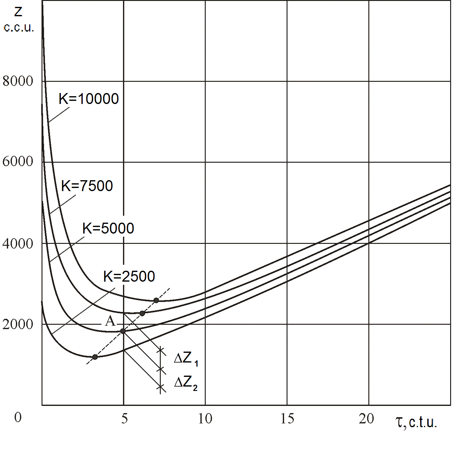
Equation (5) implies that ERSL does not depend on absolute initial costs associated with purchasing product К and the operating costs per unit С_p but depend on their relationship: the higher this ratio, the more optimal service life, and vice versa.

A decrease in product price results in a decrease in ERSL (see Figure 1 , dashed line), i.e. a cheaper product must have a shorter service life. But what is more important that there is a stiff relationship between a product price and its ERSL [see Formula (5)], which demonstrates the following: with given С_p and T _o, product price K should not be quoted in an arbitrary way; in this case, we have the so-called fair price. Let us consider this point in more detail.

As a basic dependence, we accept the dependence of the reduced costs per unit Z on time τ the product is in use at the initial costs of product purchase K = 5000 c.c.u. Minimum value Z_min is 1833 c.c.u. (See. Figure 1 ) at T _o = 5 c.c.u. Let us consider two variants of arbitrary product pricing: K = 7500 c.c.u. and K = 2500 c.c.u. In the first case, the profit is in favor of the manufacturer and the seller: ΔZ = 417 c.c.u.; in the second case ― in favor of the consumer: ΔZ = 416 c.c.u.; i.e. the first case describes dictatorship of the manufacturer; the second case ― dictatorship of the consumer. In order to have a fair (optimal) price, its value is calculated according to the formula:

$K_o=C_p{T}_o^2$ (7)

Figure 2 shows the results of calculations using Formula (4) for different С_p at constant product price K = 10.000 c.c.u.

According to the figure, the optimal service life corresponds to Z_min. The reduction in operating costs per unit results in increasing ERSL (see Figure 2 , dashed line). Let us consider the curve for С_p = 200 c.c.u ./(c.t.u.)². When Z_min is 2 653 c.c.u., T _o is 7.07 c.c.u. Let this dependence be basic (realistic) for some product. Let us assume that С_p is inaccurate because of an error made during the stage of product development due to a number of reasons. If error ΔZ₃> 0, in our example this is a curve for С_p = 300 c.c.u ./ (c.t.u.)², then we have exceeding of planned figure Z, i.e. ΔZ₃ = 710 c.c.u . In this case, the price does not meet the interests of the manufacturer and is favorable for the consumer. When С_p = 100 c.c.u ./(c.t.u.)², the manufacturer wins.

See Full Size >

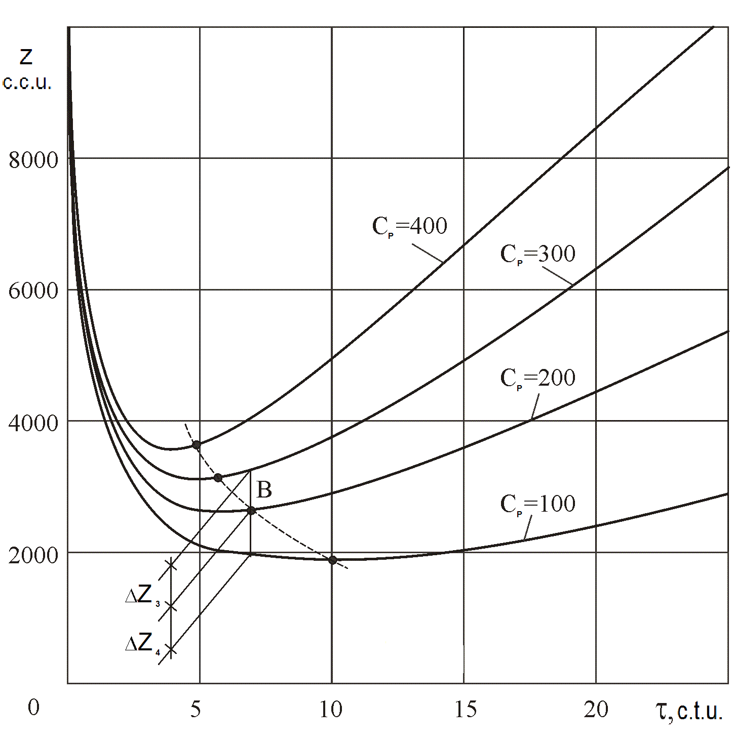
Thus, it is possible to formulate the principle for the optimal operation of any product: as to minimization of the expenditures of a consumer, a product should be used during an economically reasonable service life, the durability of which is determined by the initial costs of its purchase and ongoing operating costs(Petrushin, & Gubaydulina, 2012);

On the other hand, if the product service life is specified and operating costs per unit are estimated, then the product price is supposed to be definite in order to minimize the total costs of the manufacturer and the consumer, without prejudicing the interests of both the consumer and manufacturer. It should be optimal (fair) during the stages of manufacture and service life; so unlike competition-based pricing, pricing with respect to ERSL allows for a planning element (Chase, Equilin, & Jakob, 2001).

Let us return to basic Formula (2) for the reduced costs per unit, when the product is used, and analyze the first term. Until now, we have considered the cases with parameter $C$ being directly proportional to the time in use according to Formula (3). It is important that the operating costs per unit always depend on the time in use. In fact, if C = const, T _o = ∞, or K = 0, then the derivative of Formula (2) is equal to zero, which is absurd when applying to engineering products.

At the same time, C(τ) is determined by processes occurring in the product while it is used. It is known that the ultimate product’s failure occurs due to mechanical wear (80%), fatigue breaking (15%) and misuse (Dalsky, 1997). An action of these factors causes the product’s degradation in terms of its operational properties, i.e. degradation occurs due to the product aging. This involves increasing in the operating costs, consumables, electricity, spare parts, labor costs for maintenance and repair of the product (Franchuk, 1991; Sachko, 1997).

The table below shows the formula for parameters C(τ) and T_o . For the two latter formulae T_o is determined numerically by using the method of successive approximations.

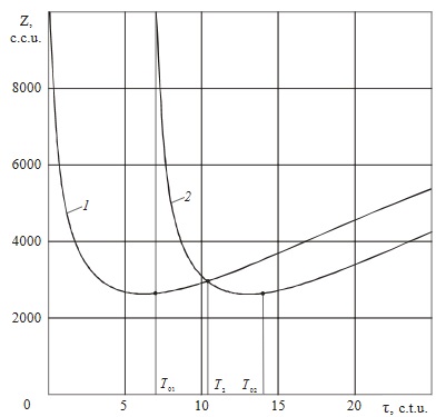
Let us consider the replacing of the old product with a new one to minimize operating costs.

Figure 3 shows the dependencies of changes in the reduced costs per unit Z on time τ when the product is used relating to old and new products. The time for replacement coincides with ERSL for old product ( T _o1). We accept that the old product is completely withdrawn from use and cannot be used. After buying a new product, the reduced costs per unit dramatically increase for the consumer, with a gradual reduction to minimum τ = T _o2. After some time, the reduced operating costs per unit relating to the new product are equal to the operating costs associated with the old product, supposing it is still in use. From that moment, the customer derives a benefit from using the new product.

See Full Size >

For the old product:

Z = С_p1τ + К₁/(τ + 1); (8)

for the new product:

Z = С_p2(τ – T _{o 1}) + К₂/(τ – T _o1 + 1), (9)

where

${\mathrm{T}}_{\mathrm{o}1}=\sqrt{{\mathrm{K}}_1/{\mathrm{C}}_{\mathrm{p}1}}$ . (10)

Time T ₂ can be determined by equaling Formulae (8) and (9):

С_p1τ + К₁/(τ + 1) – С_p2(τ – T _o1) – К₂/(τ – T _o1 + 1) = 0. (11)

To account for all possible variants, we agree on a condition that the new product is different from the old one in terms of price and ongoing operating costs:

К = n К₁; (12)

С_p2 = m С_p1. (13)

By applying Equations (12) and (13) to Formula (11) and converting the latter using Formula (10), we obtain:

(τ + 1)(τ – T _o1 + 1)[τ – m (τ – T _o1)] + T _o1 ² [τ – T _o1 + 1– n (τ + 1)] = 0 . (14)

Having solved Equation (14) with respect to τ for different values of m , n and T _o1, we determine the point of time. Obviously, the closer $T_2$ to T _o1 is (see Figure 3 ), the sooner the consumer gains from the replacement. On the other hand, under a certain combination of ongoing operating costs and the price of a new product in comparison with the old product, a variant is possible with the consumer having losses during the complete service life of the new machine.

Let us consider the case when a new product does not differ from the former relatively operating properties and design, but differs significantly in price. This corresponds to condition С_p2 = С_p1; К₂ ≠ К₁ or according to Formulae (12) and (13), $=1;n\ne 1$ . Then, Equation (14) takes the form:

(τ + 1)(τ – T _o1 + 1) + T _{o 1} [τ – T _o1 + 1– n (τ + 1)] = 0. (15)

Having solved Equation (15), we obtain:

$T_2=0.5T_{\mathrm{o}\mathrm{l}}\left(n+\sqrt{n^2+4}\right)-1$ . (16)

Figure 4 shows the results of calculations according to Formula (16) for different n . When n = 1, the old product is replaced with an equivalent product $\left(K_2=K_1\right)$ ; when $n<1$ , a cheaper product is purchased; when $n>1$ , a product is more expensive.

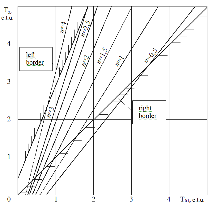
The resulting decision field has two boundaries. The right boundary corresponds to T ₂= T _o1, implying that the new product is of benefit to the customer from the point of replacement to the end of its service life. This is the case when the price of the new product is equal to the ongoing operating costs assigned to the old product at a time of its replacement, i.e. $K_2=Z_{1min}$ with $Z_{1min}$ are determined by Equation (6).

The left boundary of the decision field is obtained under condition that the consumer will gain only at the end of the new product service life, i.e. T ₂ = T _o1 + T _o2, where T _{o2 =} T _o1 $\sqrt{n}$ then:

$T_2=T_{o1}(1+\sqrt{n})$ (17)

See Full Size >

By equating (16) and (17), we obtain:

${\mathrm{T}}_{\mathrm{o}1}={\left[0.5\left(n+\sqrt{n^2+4}\right)-\sqrt{n}-1\right]}^{-1}$. (18)

By applying actual value n = К₂/К₁ to Formulae (17) and (18), we obtain coordinates of the left boundary.

Thus, the decision field is defined for the cases when products with similar operational properties, but at different prices are replaced. Obviously, the closer the time of replacement to the right boundary is, the sooner the customer derives a benefit from the new product.

Let us consider the case when the price of a new product is equal to the price of the old one, but their operational properties are different. This case has the following conditions: К₂ = К₁, С_p2 ≠ С_p1 or $n=1$, $m\ne 1$. Then using (14), we obtain:

$(\tau +\mathrm{1})\left(\tau -T_{\mathrm{o}\mathrm{1}}+\mathrm{1}\right)\left[\tau -\mathrm{m}\left(\tau -T_{\mathrm{o}\mathrm{1}}\right)\right]-T_{\mathrm{o}\mathrm{1}}^{\mathrm{3}}=\mathrm{0}$. (19)

The solution to Equation (19) for different values of $m$ specifies the field of optimal values with boundaries corresponding to T _o1 and T ₂. The optimal decision field is considerably narrower, i.e. changing in operational properties has a less influence on possible economic benefits for the consumer.

In addition to the immediate benefit from replacing, the consumer can get an absolute benefit; the value of benefit is determined by the way of comparing areas under Curves 1 and 2 in Figure 3 . Area $F_1$ from the beginning of the new product operational life ( T _o1) to point $T_3$ specifies the total expenses incurred by the consumer for using the new machine; area $F_3$ specifies the virtual operating costs associated with the use of the old machine for the same period of time. Taking integrals within T _o1 ÷ T ₃ from Equations (8) and (9), we obtain the desired areas:

$F_1=0.5{\mathrm{C}}_{p1}\left(T_3^2-T_{o1}^2\right)+{\mathrm{K}}_1\mathrm{l}\mathrm{n}|\frac{T_3+1}{T_{o1}+1}$ ; (20)

$F_2=0.5{\mathrm{C}}_{p2}\left(T_3^2-T_{o1}^2\right)-{\mathrm{C}}_{p2}{T}_{o1}\left(T_3-T_{o1}\right)+{\mathrm{K}}_2\mathrm{l}\mathrm{n}\left|T_3-T_{o1}+1\right|$. (21)

If F ₁ = F ₂, then $T_3$ defines a point of time from which the consumer starts deriving an absolute benefit from replacing the old product with a new one:

$0.5\left(T_3^2-T_{o1}^2\right)\left({\mathrm{C}}_{\mathrm{p}\mathrm{l}}-{\mathrm{C}}_{\mathrm{p}2}\right)+{\mathrm{C}}_{\mathrm{p}2}{T}_{\mathrm{o}1}\left(T_3-T_{o1}\right)+{\mathrm{K}}_1\mathrm{l}\mathrm{n}\left|\frac{T_3+1}{T_{o1}+1}\right|-{\mathrm{K}}_2\mathrm{l}\mathrm{n}\left|T_3-T_{\mathrm{o}1}+1\right|=0$. (22)

By taking Equations (12) and (13) into account and correcting by dimensionless value l = T ₃/ T _{o 1}, Equation (22) takes the form as follows:

$0.5(1-m)\left(l^2-1\right)+m(l-1)+\mathrm{l}\mathrm{n}\left|\frac{l{T}_{o1}+1}{\left(T_{o1}+1\right){\left(l{T}_{o1}-T_{o1}+1\right)}^n}\right|=0$. (23)

With replacing the old product with a similar new one having identical operational properties, i. е. under condition $=n=1$ , Equation (23) is written as follows:

$\frac{l{T}_{o1}+1}{\left(T_{o1}+1\right)\left(l{T}_{o1}+1\right)}={\mathrm{e}}^{1-l}$ . (24)

A range of $l$ values, within which the customer can have the unconditional economic benefit of the product replacement, is $1<l<2$ . When $=1$ , Equations (23) and (2) are identically satisfied. When $l=2$, Equation (24) defines upper limit $T_{o1}=3.88$ , and using Equation (23) we obtain an equation for upper limit T _o1, above which the new product will never be of benefit to the customer:

$1.5-0.5m+\mathrm{l}\mathrm{n}\left|\frac{2T_{o1}+1}{{\left(T_{o1}+1\right)}^{n+1}}\right|=0$ . (25)

Conclusion

Thus, the proposed method for optimizing the operation of a machine makes it possible not only to determine the optimal duration of its service life, but also develop an effective strategy on replacing the old machine with a new product with minimal financial losses. The results can be used as basic data for optimizing the design and manufacturing processes in mechanical engineering.

References

1. Amelkin, S.A. & Loginova, N. Yu. & Prokopiev, E.A. (2006). Determination of the optimal service life of equipment. Automaion and modern technology, 10, 3-7.
2. Chase, R. B. & Equilin, N. J. & Jakob, R. F. (2001). Production and operational management. Williams, 116-128.
3. Dalsky, M. (1997). Mechanical engineering technology. MSTU named after N.E. Bauman press, 2, 108-136.
4. Franchuk, V.I. (1991). Foundations of organizational systems. Economy, 214-218.
5. Kozlovsky, A. (2003). Production management. IFRA, 14-16, 112-126.
6. Petrushin, S. I. & Gubaidulina, R. K. & Grubiy, S. V. (2015). Optimization of Product Life Cycle. Applied Mechanics and Materials. 770, 662-669.
7. Petrushin, S.I. & Gubaydulina, R.H. (2012). New principles of mechanical engineering organization. The7thinternational Forum on Strategic Technology IFOST 2012, September 17-21, Tomsk polytechnic University. VOLUME II, 129-133.
8. Sachko, N.S. (1997). Theoretical foundations of organization of production. Minsk, Design PRO, 197-214.
9. Velikanov, K.M. (1990). Economic efficiency calculations of the new equipment. Mashinostoyeniye, 168-172, 264-286.