Study of Mathematical Models of Dynamic Systems

Abstract

It becomes necessary to describe (model) properties of a stochastic object when solving various problems of analysis and synthesis for control systems majority of modern technological, economic, biological and other objects. It is necessary to develop control systems are complex, multi-element stochastic objects for them. Linear dynamic systems (LDS) are a dominant link in the research chain. They are associated with various tasks, both regulation and control. Recently, a problem of mathematical modeling becomes essential due to the increasing need to create various control systems, as well as control systems. Nowadays, there exist some methods of mathematical models building. The efficiency of each method depends on the type of a particular problem. Therefore, one of the key problems in this field is an adequate model building, i.e., particularly versatile and simple. The authors consider a non-parametric approach to building a mathematical model of LDS based on the Duhamel integral applying stochastic approximations. The paper considers a problem of non-parametric identification and building mathematical models of stationary linear dynamic objects with delay under non-parametric uncertainty. The study of a specific class of objects with a sufficiently high degree of inertia is also carried out. The paper examines a situation when it is necessary to build a mathematical model of an object in an unstable state at the moment when observation starts.

Keywords: Dynamic system, mathematical model, initial conditions, high-order differential equation, inertia

Introduction

The paper considers a case when a researcher is forced to work with an object with relatively little information about this object. In this case, it is assumed that a researcher has only information about the qualitative behavior of the object. He is able to observe behavior of the object, and, under certain restrictions, also intentionally influences the object. The described above situations occur quite often, especially in areas of human activity where for various reasons there are no accurate models of objects, precise means of controlling the behavior of objects, as well as changes in the environment interacting with them. Resource intensity of the tasks of studying and managing objects compared with the benefits obtained by solving problems, casts doubt on the profitability of measures aimed at finding these solutions are also absent (Pervozvansky, 2017). This list can probably be continued, since the presence of a large number of factors that affect both the choice of a goal, a priori statement of the problem, search for means and methods for its solution, implementation of the solution and control of its application make it possible to talk about a large number of situations when people face similar challenges. The authors of the work offer their own ideas for solving such problems indicating specific methods for solving some of them.

Problem Statement

Suppose that in the course of an object studying (by observing this object or similar objects, as well as searching for information in sources describing the behavior of the object), a researcher has the following information (Burkov, 2017):

• object's reactions are observed when the object is stimulated by several identical input actions, slightly shifted relative to each other in time. They differ slightly from each other. This fact helps a researcher to attribute the object to the class of deterministic objects;
• response of the object to a certain input action at some moment of time differs slightly from the reaction to the same effect at another moment of time. This fact helps a researcher to attribute this object to the class of stationary objects;
• increase in the "amplitude" of the input action on the object in several times leads to an increase in the "amplitude" of the object's reaction to this effect by the same number of times. Moreover, it is useful that a sum of two or more signals stimulating the object leads to a reaction of the object, which can be quite accurately described by a sum of the object's reactions to each of these influences. Any of these facts helps a researcher to attribute the object to the class of linear objects;
• object's inertia is clearly manifested, i.e., its ability to prevent a change in its state caused by external influences. This feature of objects can also be interpreted as a significant dependence of the state (or reaction) of the object on the states of the object at previous moment of time. This fact helps a researcher to attribute the object to the class of dynamic objects;
• when a certain impact is applied to the "input" of the object, a delayed reaction of the object to this impact is observed. This fact helps a researcher to attribute the object to the class of objects with delay. Such information means that behavior of the object has qualitative properties.

Research Questions

Suppose that a researcher is able to influence the object and control the level of his influence. Thus, a researcher can compensate for the lack of information about the object that prevents the achievement of goals with satisfactory results.

We also assume that due to the restricted means of study and tools used by a researcher to describe the object, not all factors affecting the object will be taken into account in the model. The consequence of this assumption is the presence of random interference in all measurements obtained by the researcher in the course of interaction with the object. Furthermore, the authors will be guided by the assumption that a researcher does not have information about the interference or this information is not of sufficient practical value. In other words, the authors will assume that laws of distribution of random noise acting inside the object during the interaction of the object with the environment and acting in communication channels with the object are unknown (Parzen, 1962).

The last assumption is that any other information about the object and its models is not available to the researcher, or does not satisfy his goals.

A researcher can spend a lot of resources, such as computational, material, industrial, scientific and, in the end, financial resources before finding a solution under such conditions. However, modern achievements in the field of solving such problems make it possible to apply several methods for problem solving. One or another method implies the need to invest a different volume of resources for problem solving (and in the case of comparing these methods, even at the a priori stage of research, methods that are obviously more or less resource-intensive in relation to other methods can be identified) (Kazakovtsev et al., 2020; Rozhnov et al., 2021). Moreover, it is natural to assert that the choice of a method for problem solving will affect the result of its final solution and the possibility of achieving purposes set by a researcher.

Purpose of the Study

The paper considers a problem that can be defined as the purpose of researching an object. The task is to build an accurate and adequate model of the object under the conditions described above. In this case, a task of delivering values exceeding certain threshold values to the quality criteria is not set, but rather a methodology is described that can be applied to solve problems and lead to a satisfactory qualitative result in each specific area of activity and each specific task. In addition, it is supposed to apply methods that help solving a problem with small, perhaps even minimal, resource costs, while obtaining sufficiently high-quality solutions.

Research Methods

It is proposed to take as a basis the convolution model of the object’s characteristics and characteristics that affect the object and characteristics that describe the object's reactions to such influences (Xu et al., 2015). We consider models in the form of the Duhamel integral and the Cauchy-Lagrange integral (Degtyarev, 2021; Golubeva, 2021). The mathematical notation of the Duhamel integral is given in (1), the Cauchy-Lagrange integral is given in (2), and for clarity, a scalar notation of both equations is given (the case when the input actions and output responses of the object are described by one-dimensional functions of time) (Kulikovsky, 2017; Medvedev, 1975).

$x\left(t\right)={\int }_{t_0}^t{h}^{\text{'}}\left(t-\tau \right)u\left(\tau \right)d\tau$ (1)

$x\left(t\right)=f\left(t-t_0\right)+{\int }_{t_0}^t{h}^{\text{'}}\left(t-\tau \right)u\left(\tau \right)d\tau$ (2)

here x(t) is output reaction of the object observed during time t, starting from time t₀; h’(t) is the impulse-transient response of the object associated with the transient response of the object h(t) by the differentiation operator dh(t)/dt = h’(t); u(t) is an input action on the object. It leads to a change in its reaction x(t); f(t) is a free component of the object's motion, i.e., a characteristic that describes the behavior of the object in an unstable initial state. Thus, we can say that model (1) is a description of the object in a stable initial state, in contrast to model (2), which helps take into account an unstable initial state of the object.

Characteristics u(t) and x(t) can be observed in the course of experiments carried out with the object applying a variety of control tools, ranging from the senses of researchers, and control and measuring instruments, and electronic measuring sensors. Characteristics h(t) and f(t) (temporal characteristics of the object) are characteristics that identify the object itself, depend on the internal structure of the object. Furthermore, information about the behavior of these characteristics makes it possible to obtain a comprehensive description of the object's behavior. Thus, we can say that it is enough to describe the temporal characteristics of the object and use these descriptions when searching for a model, as shown in (1) and (2) in order to build a model of the object under the conditions defined above.

One of the simplest and most illustrative methods for describing the temporal characteristics of the object (identification of the object) is a method based on observing the behavior of an object under conditions when the object is affected by special test actions. Everyone can get acquainted with the description of several similar methods in the reference book. In this paper, the authors consider a method of temporal characteristics. It involves the impact on the object using the characteristic u(t) in such a way that at the "output" of the object reactions x(t) are observed corresponding to the temporal characteristics of the object h(t) (or h'(t) and f(t).

So, it is necessary to apply a test signal to the “input” of the object, which is described by the Heaviside function 1(t) in order to find a description of the transient response of the object applying a method of time characteristics (Priestley & Chao, 1972). At the output of the object, a reaction will be observed that approximately repeats the behavior of the transient response of the object. Figure 1 illustrates this experiment.

See Full Size >

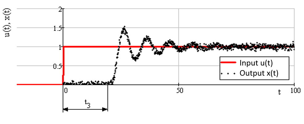
Figure 1 demonstrates a characteristic u(t) acting on the object (solid line) and a reaction of the object to the impact x(t) (depicted on the graph by dots). When entering an "input" of the object of influence, there is a delayed reaction of the object to this impact, the delay time of the object is indicated as t₃. Besides, according to the experiment demonstrated in Figure 1, one can notice the presence of random noise that affects the measurements of the object's response. It is a problem that a researcher will inevitably face.

The paper states that it is enough to bring the object into the desired unstable initial state, followed by the termination of the impact on the object to describe the behavior of the free component of the object's motion. So, at the "input" of the object, the reaction of the object will be observed, approximately repeating a free component of the object's movement. Figure 2 in the graph presents an illustration of the experiment in identifying a free component of the object's motion.

See Full Size >

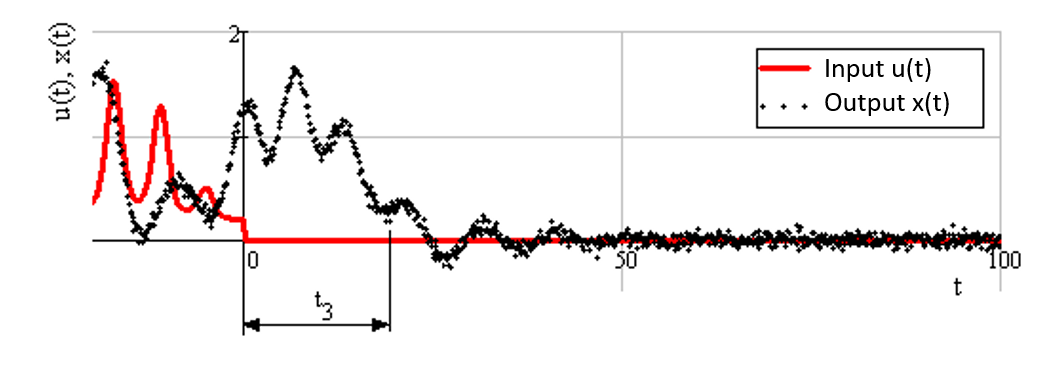
Figure 2 demonstrates how the object is directed to the unstable initial state with the help of the input action u(t) in the time interval less than the time t=0. Then, in the time interval from the moment t=0 to t=100, the impact on the object stops and at the “output” of the object, there is a reaction of the object x(t) lagging in time by t₃, corresponding to a free component of the object’s motion describing the object in this unstable initial state.

We can proceed to building a model of the object in the form (1) and (2) having restored the behavior of the temporal characteristics of the object according to the observations of these characteristics obtained as a result of experiments with the object.

The paper proposes to apply methods of non-parametric statistics and, in particular, nonparametric Nadarai-Watson estimates, and Priestley estimates to restore the behavior of time characteristics (Medvedeva, 1995; Nadaraya, 1965). The application of these methods is due to the fact that the researcher is in conditions of non-parametric uncertainty, does not contain a priori information that makes it possible to find a parametric description of the characteristics of the object with limited resources. Moreover, the paper proposes to apply modified Priestley regression estimates. They help find a description of the impulse response of an object from observations of the transition response.

The authors suggest to apply the modified Priestley estimate to find a description of the impulse transient response of an object. The resulting estimate is given in (3).

$h_s^{\text{'}}\left(t\right)={\left[s\cdot {\left(c_s^h\right)}^2\right]}^{-1}{\sum }_{i=1}^{s}h\left(t_i\right)\cdot H^{\text{'}}\left(\left(t-t_i\right)/c_s\right)$ (3)

here $h_s^{\text{'}}\left(t\right)$ is a non-parametric estimate of the object's transient response built from a sample of values of the object's transient response h(t_i), at time moment t_i, s is a sample size of values h(t_i), c_s^h is the blur parameter (Tsypkin, 1970) of the non-parametric estimate (3), H(∙) is a bell-shaped function of the nonparametric estimate.

It is proposed to apply nonparametric Nadaraya-Watson estimates to describe a free component of the motion of an object. The resulting estimate is presented in (4).

$f_s\left(t\right)={\left[s\cdot c_s^f\right]}^{-1}{\sum }_{i=1}^{s}f\left(t_i\right)\cdot H\left(\left(t-t_i\right)/c_s\right)$ (4)

here $f_s\left(t\right)$ is the non-parametric estimate of the free component of the object's motion, f(t_i) is the value of the free component of the object's motion at time t_i, c_s^f is the blur parameter of the non-parametric estimate (4).

The estimates application (3) and (4) for the temporal characteristics of the object description makes it possible to build a model of the output characteristic of the object:

$x_s\left(t\right)=f_s\left(t-t_0\right)+{\int }_{t_0}^t{h}_s^{\text{'}}\left(t-\tau \right)\cdot u\left(\tau \right)d\tau$ (5)

here $x_s\left(t\right)$ is a non-parametric model of the object's response to the input action u(t).

The authors suggest to apply criteria as an error in modeling the output response of the object (6) that describes the deviation of the response of the model from the response of the object under the same conditions. It is needed for the quality of the obtained model’s estimate., The paper proposes to apply the average absolute relative error of modeling the object's output reaction as a criterion that reflects the quality of the model in relative terms. They are better for a researcher to assimilate and estimate (7).

$Q_1=s^{-1}{\sum }_{i=1}^s{\left(x\left(t_i\right)-x_s\left(t_i\right)\right)}^2$ (6)

$Q_2=s^{-1}{\sum }_{i=1}^s\left|\left(x\left(t_i\right)-x_s\left(t_i\right)\right)/x\left(t_i\right)\right|\cdot \text{100\%}$ (7)

here $x\left(t_i\right)$ is the value of the output characteristic of the object at time t_i (Hollander & Wolfe, 1999).

Findings

The authors select a specific class of objects characterized by a high degree of inertia to demonstrate the operation of the proposed algorithm. In other words, we can say that such objects can be described by high-order differential equations. The reason for selecting such a class of objects is to study the applicability of the proposed method for building models of such objects that are rather difficult for description.

We decided to apply a parametric model of the object as the modeling object. It is given in the form of a tenth-order differential equation (8), implemented on a computer. Further, we call this model as an object, i.e., its imitation, developed to demonstrate the operation of the method (Efimova et al., 2017; Eliseeva & Yuzbashev, 2017).

$\begin{array}{c}\frac{d^{\text{10}}}{{\text{dt}}^{\text{10}}}x\left(t\right)+0\text{.7636}\frac{d^9}{{\text{dt}}^9}x\left(t\right)+4\text{.0512}\frac{d^8}{{\text{dt}}^8}x\left(t\right)+2\text{.3679}\frac{d^7}{{\text{dt}}^7}x\left(t\right)+6\text{.3677}\frac{d^6}{{\text{dt}}^6}x\left(t\right)\\ +2\text{.7259}\frac{d^5}{{\text{dt}}^5}x\left(t\right)+\\ +4\text{.8623}\frac{d^4}{{\text{dt}}^4}x\left(t\right)++1\text{.3807}\frac{d^3}{{\text{dt}}^3}x\left(t\right)+1\text{.8037}\frac{d^2}{{\text{dt}}^2}x\left(t\right)+\\ 0\text{.2596}\frac{d}{\text{dt}}x\left(t\right)+0\text{.2596}x\left(t\right)=u\left(t-t_3\right)\end{array}$

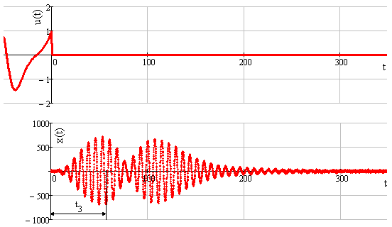
Bring the object to the needed state with the subsequent termination of the impact on the object to describe an object under conditions of an unstable initial state. At the output, the reaction of the object is observed. It corresponds to the free component of the object's motion. The values of the input and output characteristics of the object are observed with equal time delays, so that the total amount of characteristic values is 5000. At the output, the reaction of the object with random additive noise is observed. Its intensity is equal to 5% of the amplitude of the object’s reaction. The results of the experiment are demonstrated in Figure 3.

See Full Size >

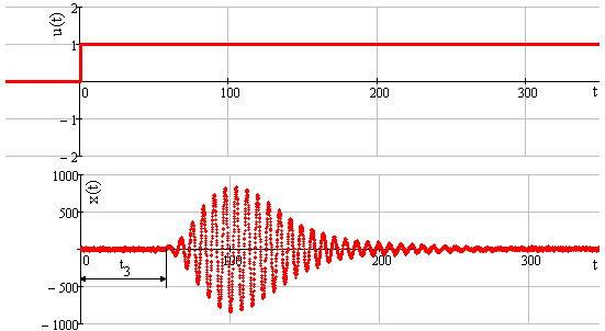
Then, the impact corresponding to the Heaviside function is applied to the input of the object in the “calmed down” state, the reaction of the object is observed at the output, corresponding to the transient response of the object. Similar to the previous experience, 5000 values of the input and output characteristics of the object were measured. Moreover, at the “output” of the object, values with additive noise with an intensity of 5% relative to the amplitude of the output response of the object are observed. Figure 4 illustrates this experiment.

See Full Size >

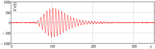
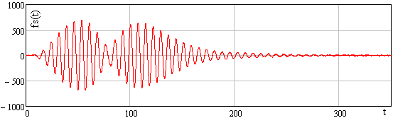
Further, according to expressions (3) and (4), with parameters csh=0.7, csf=0.35, H(t)=[(cos(πt)+1)/2]∙[1(t+1)-1(t-1)] (1(t) is Heaviside function) a non-parametric description of the temporal characteristics of the object was found. Graphs of the obtained non-parametric estimates are given in Figure 5 and Figure 6.

See Full Size >

See Full Size >

The authors built a non-parametric model of the object with the help of the expression (5). It makes it possible to describe the reaction of the object to an arbitrary input action taking into account the unstable initial state of the object.

The next experiment compared the obtained non-parametric model of the object with the reaction of the object itself (given in the form of a differential equation). We compared them applying criteria (6) and (7), the reactions of the object and the model to the same input action. The “input” of the object and the “input” of the model are subjected to the action demonstrated in Figure 7. Corresponding reactions are recorded at the "output" of the object and at the "output" of the model. Both of these reactions are also demonstrated in Figure 7.

See Full Size >

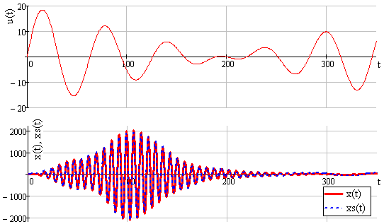
The values of the quality criteria of the obtained model of the object were Q₁≈1000 and Q₂≈20% respectively. These indicators state that the resulting model has significantly moved away from the object’s indicators. However, the obtained quality of the model turns out to be satisfactory in conditions when a researcher does not have practically any information for studying and forming hypotheses regarding the object of research.

Such, at first glance, poor modeling results indicate that there are still a lot of unsolved (or insufficiently solved) problems in the field of such objects studying. However, if we take into account that the solved problem of building object’s models with a high degree of inertia can, no doubt, be classified as complex and resource-intensive tasks. If we take into account that the conditions under which the problem was solved can generally turn out to be an insurmountable obstacle to solving this problem for a lot of trained and experienced researchers, then the results obtained seem significant, considering both theoretical methods developments, and applied applications for solving such problems. Moreover, the authors emphasize the fact that applied methods do not require a large amount of high-quality information. This fact indicates a low resource intensity of the method, an insignificant level of costs for solving problems applying a proposed method.

Conclusion

The obtained results help conclude that it is possible to describe objects belonging to the class of stationary linear dynamic objects with delay and a high degree of inertia under conditions of uncertainty. The relevance of the obtained results supposes new opportunities to study the world around us, and the possibilities of its development in areas where it was simply impossible or excessively expensive. Non-parametric models of objects make it possible for researchers to build hypotheses and assumptions about the studied objects, improve models up to the achievement of these models at the level of fundamental laws. Moreover, non-parametric models, however, like any others, can be a basis for solving other problems that include decision support problems at controlling objects, or problems of direct control by these objects.

Acknowledgments

This work was supported by the Ministry of Science and Higher Education of the Russian Federation (Grant No.075-15-2022-1121).

References

• Burkov, V. N. (2017). Fundamentals of mathematical theory for active systems. Nauka.

• Degtyarev, V. G. (2021). Mathematical modeling: textbook. PGUPS.

• Efimova, M. R., Ganchenko, O. I., & Petrova, E. V. (2017). Workshop on the general theory of statistics: Training guide. Finance and statistics.

• Eliseeva, I. I., & Yuzbashev, M. M. (2017). General theory of statistics: Textbook. Finance and statistics.

• Golubeva, N. V. (2021). Mathematical modeling of systems and processes: study guide for universities. Lan'.

• Hollander, M., & Wolfe, D.A. (1999). Non-parametric statistical methods. Wiley.

• Kazakovtsev, L., Rozhnov, I., Popov, A., & Tovbis, E. (2020). Self-Adjusting Variable Neighborhood Search Algorithm for Near-Optimal k-Means Clustering. Computation, 8(4), 90.

  Google Scholar

  Crossref

• Kulikovsky, R. (2017). Optimal adaptive processes in automatic control systems. Nauka.

• Medvedev, A. V. (1975). Identification and control for linear dynamic systems of unknown order. Optimization Techniques IFIP Technical Conference (pp. 48-55). Springer – Verlag.

  Google Scholar

  Crossref

• Medvedeva, N. A. (1995). Nonparametric models and controllers. Russian Physics Journal, 38(9), 978-982.

  Google Scholar

  Crossref

• Nadaraya, E. A. (1965). Non-parametric Estimates of the Regression Curve. Proceedings of VU AN GrSSR. 5, 55-68.

  Google Scholar

  Crossref

• Parzen, E. (1962). On Estimation of a Probability Density Function and Mode. The Annals of Mathematical Statistics, 33(3), 1065-1076.

  Google Scholar

  Crossref

• Pervozvansky, A. A. (2017). Mathematical models in production management. Nauka.

• Priestley, M. B., & Chao, M. T. (1972), Non-Parametric Function Fitting. Journal of the Royal Statistical Society: Series B (Methodological), 34, 385-392.

  Google Scholar

  Crossref

• Rozhnov, I. P., Kazakovtsev, L. A., & Karaseva, M. V. (2021). Informative Features Selection for Building an Optimization Model of the Aluminum Electrolytic Cell Thermal Regime. Revista geintec-gestao inovacao e tecnologias, 11(4), 605-622.

• Tsypkin, Y. Z. (1970). Fundamentals of the learning systems theory. Nauka.

• Xu, X., Yan, Z., & Xu, S. (2015). Estimating wind speed probability distribution by diffusion-based kernel density method. Electric Power Systems Research, 121, 28-37.

  Google Scholar

  Crossref