
Disk Drives Remaining Useful Life Prediction Using the Extreme Learning Machine


Abstract
The article deals with the problem of predicting the remaining useful life of disk drives using a machine learning model, in particular, using an Extreme Learning Machine (ELM). A method is proposed for improving the values of model quality metrics by generating new features, as well as their selection using a method that implements the calculation of the symmetric Kullback-Leibler Divergence (SKLD). It is shown that a model based on an extreme learning machine and trained on the basis of a dataset formed from the results of generation of new features and their subsequent selection by the SKL method can predict the remaining useful life with an average error of 2.5 days, while model training time is about 6 seconds. The results of a comparative analysis are presented, confirming the efficiency of the proposed model based on ELM. Additionally, the methods for generating features BY and MI are compared, and their shortcomings over SKLD in this case are demonstrated.
Keywords: Multidimensional time series, predicting, decision tree, random forest, feature engineering, remaining useful life
Introduction
Today, in any computer system, whether it is a regular personal computer or a large computing center, data drives on hard or solid-state media are used. Every year, the volume of processed information becomes larger and the growth in 2020 compared to 2019 was already 33% (Gantz & Reinsel, 2012). This pace is taking its toll on data centers around the world, leading to multiple drive failures. With this problem, the task of diagnosing disk and solid-state drives appeared.
To simplify the diagnosis of data drives, manufacturers equip them with self-monitoring, analysis and reporting technology (SMART, Self-Monitoring, Analysis and Reporting Technology). A self-monitoring system consists of a set of sensors, each of which monitors a certain characteristic of the drive during its operation. For example, it can be the number of writes, reads, bad sectors, etc. Each sensor can report the measured characteristic to the operator who requested it. Usually, such an operator is a program that has access to the data drive (Aussel et al., 2017; Bagul, 2009; Lu et al., 2020).
Since there are many drives in the data center, the status of each of which needs to be monitored, special monitoring systems are created that collect performance data from all storage devices. This is a huge amount of information that can exceed terabytes. So, for example, BackBlaze posted a report for 2020, where they provided statistics on almost 163 thousand disk drives, 1302 of which failed. In this case, the average disk life cycle time was 25 months (Klein, 2021).
Problem Statement
It is difficult for a person to independently analyze such a volume of data, so we came up with approaches that allow us to obtain the remaining useful life of a disk drive (Remaining Useful Life, RUL), which can be conditionally divided into two types. The first involves using multiple sensor metrics in a single formula that results in a rough RUL score. This approach is used, for example, by Samsung (Li et al., 2019). The second, which is considered more advanced, uses machine learning algorithms (Basak et al., 2019; Demidova & Fursov, 2021; Xu et al., 2016). Its advantage lies in the fact that, when calculating, the model can take into account the degree of influence of each sensor on the final RUL value, as well as hidden patterns in the data, which may consist in the indirect influence of the indicator of one sensor on another (Anantharaman et al., 2018; Andrianova et al., 2020).
Recurrent networks are the most efficient of all machine learning algorithms in terms of decision accuracy in the remaining life prediction problem. Such superiority is due to the use of a built-in memory mechanism, thanks to which the model is able to learn based on its previous experience (Demidova & Gorchakov, 2022a; Wang et al., 2019). However, if the size of the dataset used to train the model is very large and the architecture of the model is multi-layered, then the training process can be very long. The ELM network differs from the recurrent network in its simplicity and a different approach to the learning mechanism, which consists in calculating the inverse Moore-Penrose matrix, which ultimately provides a higher learning rate, with slightly less good quality metrics calculated during training (Dubnov, 2018; Huang et al., 2004).
Research Questions
In the course of the study, it is supposed to consider a number of aspects related to the questions of increasing the speed in the decision-making process and extracting additional information hidden in the readings of smart sensors. In particular, it is planned to explore such questions as:
- Using of ELM networks in predicting the remaining useful life of disk drives based on some dataset, the feature values in which are generated based on the readings of SMART sensors;
- Selection by the SKLD (Symmetric Kullback-Leibler Divergence) method of features from among those generated based on the readings of SMART sensors.
- Evaluation and comparative analysis of the quality of predicting the remaining useful life of disk drives based on datasets generated both on the basis of SMART sensor readings and using new generated features.
Purpose of the Study
The purpose of the study is to develop an ELM model capable of predicting the remaining useful life of disk drives with the lowest possible error.
Research Methods
Extreme learning machine
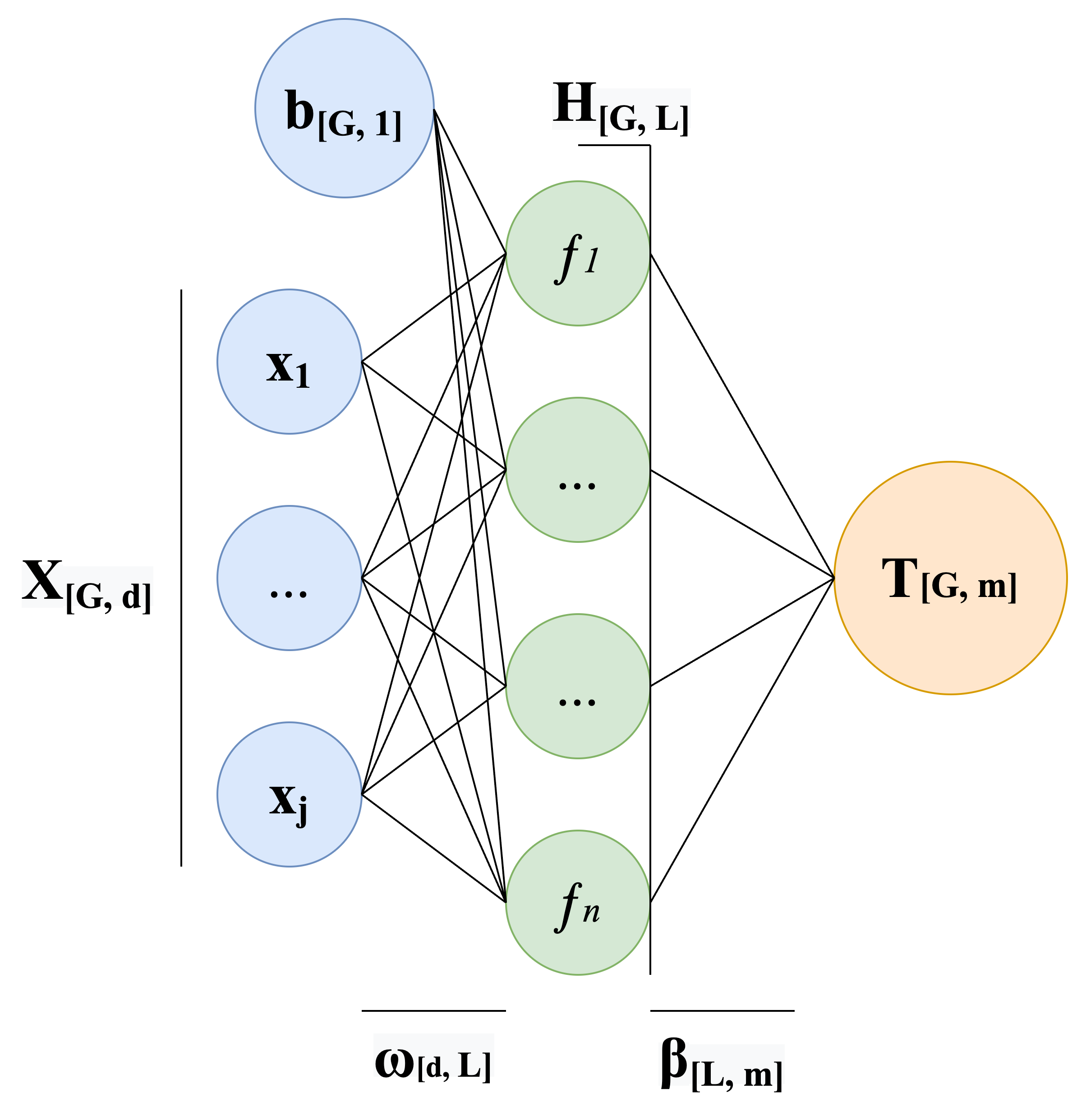
The ELM network uses the Moore-Penrose inversion (Demidova & Marchev, 2019; Huang et al., 2004), due to which the entire architecture of the final neural network consists of one hidden layer. This allows you to increase the learning rate. The output vector of ELM network is calculated as:
(1)
where – number of hidden neurons, – input data vector, – weight vector between the hidden layer and the output, – weight vector between the input and the hidden layer, – activation function, – bias vector.
Expression (1) can be written as
,
where
,
where – dimension of the component of the output vector; – output matrix of the hidden layer of the neural network; – output vector, – pseudo-inverse matrix defining the connection between the hidden layer and the output vector (Huang et al., 2004).
In general, the learning process of an ELM network can be described as follows (Demidova & Gorchakov, 2022b):
- randomly determine weights ωb and biases bbb=1,L¯;
- calculate the output matrix H;
- calculate the output matrix β=H†T, where H†=HTH-1HT;
- use the output matrix β to predict the output vector T=Hβ.
The neural network architecture based on the extreme learning machine is shown in Figure 1.
Dataset
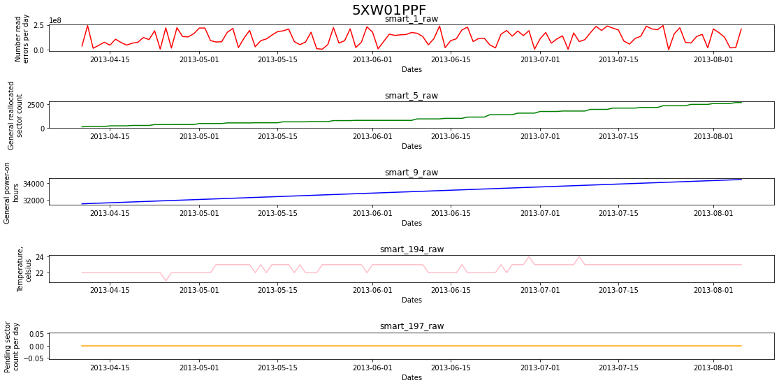
When performing experiments, we used a data set for 2013 from BackBlaze, which contains data for 8 months on 35,000 disk drives (BackBlaze, 2018). At the same time, the readings of only five representative SMART sensors were considered, the list of which is given in Table 1. The readings of the SMART sensors of each disk drive were used in aggregate in the form of a multidimensional VR. Figure 2 shows an example of such a VR for one of the disk drives.
Feature engineering
Different disk drives can have significantly different ranges of change in sensor readings for each feature, which can lead to a distorted perception of data by the model. In this regard, it was decided to apply standardization (Serneels et al., 2006) to the values of sensor readings for each feature.
The remaining useful life of a disk drive, RUL, acts as a target variable and is not contained in the data set, but can easily be calculated based on the number of records for a particular disk drive, since one reading of the disk drive sensor corresponds to one day (Demidova & Fursov, 2022; Wang et al., 2019).
In the course of the research, an experiment was carried out to develop a forecasting model, which involved a data set of 5 initial time series with generated features. In addition, 50 features were generated, fixing, in particular, the minimum and maximum values of the original time series, the number of maximum and minimum peaks of the original time series, the most frequently repeated values of the original time series, as well as some other statistical characteristics. In order to select the most informative and non-correlated features from 50 generated features, a selection procedure was performed.
Feature selecting
When implementing the selection procedure, the method was used, based on the calculation of the symmetric distance (Kullback-Leibler Divergence) (Cover & Thomas, 1991; Dubnov, 2018), used to determine the proximity of the distribution functions of various random variables.
When solving the problem of dimensionality reduction based on the Kullback-Leibler divergence, it is advisable to use the difference in the probability density functions of the vectors corresponding to the values of the feature ( ) and the target variable as a feature selection criterion. The distance value characterizes the proximity of the distributions of the values of the feature ( ) relative to the distribution of the target variable . The larger the value of the distance, the less similar these distributions are, and vice versa, the smaller the value of the distance, the greater the similarity between the distributions, which indicates that the considered-th feature ( ) is not informative.
Distance is defined as:
where is the-th component of the vector containing the values of the probability density function for the vector of the-th feature , is the-th component of the vector containing the values of the probability density function for the target feature vector .
Since the distance is asymmetric, that is, , in practice, a symmetrical version is usually used for the Kullback-Leibler Divergence ():
(2)
The condition for selecting a feature when applying the method was that the values of proximity measures (2) fall into the range between the 3rd and 4th quartiles. In the problem under consideration, using the method, 15 features were selected out of 50 generated.
Data splitting
In each experiment, the data set was transformed in such a way as to obtain an array , consisting of subarrays , where is the ordinal number of the subarray. In this case, a certain number of days , was selected, which was used as a sliding window when scanning a multivariate time series with . This window moved through the entire history of each disk drive and made it possible to compile a set of matrices with dimension , where is the number of features. The total number of subarrays for a particular disk drive was calculated as:
where is the total number of observation days for a particular disk drive.
Metrics
The (Mean Squared Error) metric was chosen as the loss function:
for a visual interpretation of the results, the (Root Mean Squared Error) metric was used:
where is the number of predicted values of the RUL parameter; is the true value of the-th element of the vector of the target variable; is the predicted value of the-th element of the target variable vector.
Both metrics are minimized during training.
Findings
The development of forecasting models was carried out in the environment in Google Colab using Python 3.10.
The training time of the ELM model using the original dataset (i.e., the set without feature generation) and the dataset with generated and selected features is presented in Table 2.
Table 3 presents the values of model quality metrics on the original data set and the data set with generated and selected features. The RMSE indicator can be interpreted as the number of days by which the model was wrong.
Conclusion
Based on the data in tables 2 and 3, we can conclude that the model based on the ELM network learned quickly, while having good quality metrics after feature selection. It should be noted that in the course of the experiments, 2 more methods of feature selection were considered - the Benjamini-Yekutieli procedure (BY) and the method based on mutual information (Mutual Information, MI) (Dubnov, 2018). However, their use turned out to be less effective than the use of the SKLD method. The BY method selected 40 features, while the values of the MSE and RMSE metrics of the model built on their basis were comparable to the values of the same metrics for the model for which the features were selected by the SKL method, but learning was almost 2 times slower. The MI method selected 15 features that differed from those chosen by the SKLD method, while the values of the MSE and RMSE metrics turned out to be worse than in the case of working with the SKLD method, namely, 20% and 10% more, respectively.
The article considers the solution of the problem of predicting the remaining useful life of disk drives using a model based on the ELM network, while showing the effectiveness of using such a model in the problem under consideration. In addition, it was concluded that it is possible to improve the quality of the model in the case of selection by the SKLD method of features from among those generated based on the readings of SMART sensors.
Further research considers the idea of optimizing the generation of random weights and bias also building metamodels to improve MSE and RMSE metrics.
References
Anantharaman, P., Qiao, M., & Jadav, D. (2018). Large scale predictive analytics for hard disk remaining useful life estimation. In 2018 IEEE International Congress on Big Data (BigData Congress) (pp. 251-254). IEEE.
Andrianova, E. G., Golovin, S. A., Zykov, S. V., Lesko, S. A., & Chukalina, E. R. (2020). Review of modern models and methods of analysis of time series of dynamics of processes in social, economic and socio-technical systems. Russian Technological Journal, 8(4), 7-45.
Aussel, N., Jaulin, S., Gandon, G., Petetin, Y., Fazli, E., & Chabridon, S. (2017, December). Predictive models of hard drive failures based on operational data. In 2017 16th IEEE International Conference on Machine Learning and Applications (ICMLA) (pp. 619-625). IEEE.
BackBlaze. (2018). dataset https://www.backblaze.com/b2/hard-drive-test-data.html
Bagul, Y. G. (2009). Assessment of current health and remaining useful life of hard disk drives [Master‘s Thesis]. Northeastern University, Boston, MA.
Basak, S., Sengupta, S., & Dubey, A. (2019). Mechanisms for integrated feature normalization and remaining useful life estimation using lstms applied to hard-disks. In 2019 IEEE international conference on smart computing (SMARTCOMP) (pp. 208-216). IEEE.
Cover, T. M., & Thomas, J. A. (1991). Elements of information theory. John Wiley and Sons Ltd.
Demidova, L., & Fursov, I. (2022). Software implementation of neural recurrent model to predict remaining useful life of data storage devices. In High-Performance Computing Systems and Technologies in Scientific Research, Automation of Control and Production: 11th International Conference, HPCST 2021, Barnaul, Russia, May 21–22, 2021, Revised Selected Papers (pp. 391-400). Springer, Cham.
Demidova, L. A., & Fursov, I. A. (2021, November). Aspects of Feature Engineering in the Problem of Predicting the Service Life of Hard Drives. In 2021 3rd International Conference on Control Systems, Mathematical Modeling, Automation and Energy Efficiency (SUMMA) (pp. 1188-1191). IEEE.
Demidova, L. A., & Gorchakov, A. V. (2022a). Application of bioinspired global optimization algorithms to the improvement of the prediction accuracy of compact extreme learning machines. Russian Technological Journal, 10(2), 59-74.
Demidova, L. A., & Gorchakov, A. V. (2022b). Classification of Program Texts Represented as Markov Chains with Biology-Inspired Algorithms-Enhanced Extreme Learning Machines. Algorithms, 15(9), 329.
Demidova, L. A., & Marchev, D. V. (2019). The use of recurrent neural networks in the problems of classifying the discovery of complex technical systems in the framework of proactive maintenance. Bulletin of the Ryazan State Radio Engineering University, 69, 135-148.
Dubnov, J. A. (2018). On entropy criteria for feature selection in data analysis problems. ITiVS, 2, 60-69. [In Russ.]
Gantz, J., & Reinsel, D. (2012). The Digital Universe in 2020: Big Data, Bigger Digital Shadows, and Biggest Growth in the Far East. IDC iView: IDC Analyze the Future.
Huang, G. B., Zhu, Q. Y., & Siew, C. K. (2004). Extreme learning machine: a new learning scheme of feedforward neural networks. In 2004 IEEE international joint conference on neural networks (IEEE Cat. No. 04CH37541) (Vol. 2, pp. 985-990). IEEE.
Klein, A. (2021, January 26). Backblaze Hard Drive Stats for 2020. https://www.backblaze.com/blog/backblaze-hard-drive-stats-for-2020
Li, Q., Li, H., & Zhang, K. (2019). A survey of SSD lifecycle prediction. In 2019 IEEE 10th International Conference on Software Engineering and Service Science (ICSESS) (pp. 195-198). IEEE.
Lu, S., Luo, B., Patel, T., Yao, Y., Tiwari, D., & Shi, W. (2020). Making disk failure predictions SMARTer. 18th USENIX Conference on File and Storage Technologies (FAST 20), 151-167.
Serneels, S., De Nolf, E., & van Espen, P. J. (2006). Spatial sign preprocessing: A simple way to impart moderate robustness to multivariate estimators. Journal of Chemical Information and Modeling, 46(3), 1402-1409.
Wang, Q., Zheng, S., Farahat, A., Serita, S., & Gupta, C. (2019). Remaining useful life estimation using functional data analysis. In 2019 IEEE international conference on prognostics and health management (icphm) (pp. 1-8). IEEE.
Xu, C., Wang, G., Liu, X., Guo, D., & Liu, T.-Y. (2016). Health Status Assessment and Failure Prediction for Hard Drives with Recurrent Neural Networks. IEEE Transactions on Computers, 65(11), 3502-3508.
Copyright information

This work is licensed under a Creative Commons Attribution-NonCommercial-NoDerivatives 4.0 International License
About this article
Publication Date
27 February 2023
Article Doi
eBook ISBN
978-1-80296-960-3
Publisher
European Publisher
Volume
1
Print ISBN (optional)
-
Edition Number
1st Edition
Pages
1-403
Subjects
Hybrid methods, modeling and optimization, complex systems, mathematical models, data mining, computational intelligence
Cite this article as:
Demidova, L. A., & Fursov, I. A. (2023). Disk Drives Remaining Useful Life Prediction Using the Extreme Learning Machine. In P. Stanimorovic, A. A. Stupina, E. Semenkin, & I. V. Kovalev (Eds.), Hybrid Methods of Modeling and Optimization in Complex Systems, vol 1. European Proceedings of Computers and Technology (pp. 304-312). European Publisher. https://doi.org/10.15405/epct.23021.37