A Neutrosophic Adaptive Recurrent Neural Network for Time-Varying Matrix Inversion

The Neutrosophic logic controller

The entries of a neutrosophic set $\mathcal{K}$ are neutrosophic numbers of the next form (Smarandache, 2003):

$\mathcal{K}=\left\{\langle x:T_{\mathcal{K}}\left(x\right),I_{\mathcal{K}}\left(x\right),F_{\mathcal{K}}\left(x\right)\rangle |x\in \mathcal{U}\right\},$ (4)

where $T_{\mathcal{K}}\left(x\right),I_{\mathcal{K}}\left(x\right)$, and $F_{\mathcal{K}}\left(x\right)$, respectively, denote the truth, the indeterminacy, and the falsity membership functions whose values are independent and within $\left[\mathrm{0,1}\right]$. In the NSZNN design, the varying-gain parameter ${\lambda }^{\nu }$ values will be viewed as predictions according to the $T_{\mathcal{K}}\left(x\right),I_{\mathcal{K}}\left(x\right)$, and $F_{\mathcal{K}}\left(x\right)$ values. Since the main objective in the ZNN design is $E\left(t\right)=\mathbf{0}$, it makes sense to employ $\mathrm{\eta }:=\parallel E\left(t\right){\parallel }_F$ as a metric for developing NSLC in the NSZNN design. Note that ${‖\cdot ‖}_F$ signifies the matrix Frobenius norm.

In our approach, the NSLC's development is divided into three stages. These stages are the neutrosophication process, the neutrosophic inference engine, and the de-neutrosophication process.

In the neutrosophication process, the input set is transformed into the fuzzy input set $\mathcal{J}$ and the output set is transformed into the fuzzy output set $\mathcal{G}=\{T_{\mathcal{K}},I_{\mathcal{K}},F_{\mathcal{K}}\}$, which is in the neutrosophic format, through the neutrosophication process. It is important to note that the truth, indeterminacy, and falsity membership functions are defined as sigmoid, Z-shaped, and Gaussian functions. Particularly, we consider the following sigmoid truth-membership function:

$\mathrm{T}\left(\mathrm{\eta }\right)=\mathrm{1}/(\mathrm{1}+{\mathrm{e}}^{-a_{\mathrm{1}}(\mathrm{\eta }-a_{\mathrm{2}})}).$ (5)

where the parameters $a_{\mathrm{1}}$ and $a_{\mathrm{2}}$, respectively, are responsible for its slope at the crossover point $\eta =a_{\mathrm{2}}$, Further, we consider the next Z-shaped falsity-membership function:

$\mathrm{F}\left(\mathrm{\eta }\right)=\left\{\begin{array}{ll}\mathrm{1},& \mathrm{\eta }\le s_{\mathrm{1}}\\ \mathrm{1}-\mathrm{2}{\left(\frac{\mathrm{\eta }-s_{\mathrm{1}}}{s_{\mathrm{2}}-s_{\mathrm{1}}}\right)}^{\mathrm{2}},& s_{\mathrm{1}}\le \mathrm{\eta }\le \frac{s_{\mathrm{1}}+s_{\mathrm{2}}}{\mathrm{2}}\\ \mathrm{2}{\left(\frac{\mathrm{\eta }-s_{\mathrm{2}}}{s_{\mathrm{2}}-s_{\mathrm{1}}}\right)}^{\mathrm{2}},& \frac{s_{\mathrm{1}}+s_{\mathrm{2}}}{\mathrm{2}}\le \mathrm{\eta }\le s_{\mathrm{2}}\\ \mathrm{0},& \mathrm{\eta }\ge s_{\mathrm{2}}\end{array}\right.,$ (6)

where the parameters $s_{\mathrm{1}}$ and $s_{\mathrm{2}}$, respectively, signify the shoulder and the foot of the function. Lastly, we consider the next Gaussian indeterminacy-membership function:

$\mathrm{I}\left(\mathrm{\eta }\right)={\mathrm{e}}^{-\frac{(\eta -d_{\mathrm{2}}{)}^{\mathrm{2}}}{\mathrm{2}{d}_{\mathrm{1}}^{\mathrm{2}}}},$ (7)

where the parameters $d_{\mathrm{1}}$ and $d_{\mathrm{2}}$, respectively, signify the standard deviation and the mean.

In the neutrosophic inference engine, the next "IF-THEN" rule is considered as the neutrosophic rule between $\mathcal{J}$ and $\mathcal{G}$ :

$R:\mathrm{}\mathrm{}\mathrm{I}\mathrm{f}\mathrm{}\mathrm{}\mathcal{J}=\mathrm{S}\mathrm{E}\mathrm{}\mathrm{}\mathrm{t}\mathrm{h}\mathrm{e}\mathrm{n}\mathrm{}\mathrm{}\mathcal{G}=\{T_{\mathcal{K}},I_{\mathcal{K}},F_{\mathcal{K}}\},$

where $\mathrm{S}\mathrm{E}$ is a fuzzy set, and exactly indicates a significant error.

In the neutrosophication process, the conversion $\langle \eta :T\left(\eta \right),I\left(\eta \right),F\left(\eta \right)\rangle \to \nu (\eta ,t)\in \mathbb{R}$ results to a single (crisp) value $\nu (\eta ,t)$. Particularly, the following de-neutrosophication rule is proposed to obtain the parameter $\nu (\eta ,t)$:

$\nu (\eta ,t)=r_{\mathrm{1}}+r_{\mathrm{2}}\frac{T\left(\eta \right)+I\left(\eta \right)+F\left(\eta \right)}{t+\mathrm{1}},$(8)

where $t\in {\mathbb{R}}_{\mathrm{0}}^{+}$, and $r_{\mathrm{1}}\ge \mathrm{1}$ and $r_{\mathrm{2}}\ge \mathrm{0}$ are parameters for setting the lower and upper limit of (8), respectively.

Solving the TV-MI problem through the ZNN and NSZNN designs

Considering the TV-MI problem (3), the next ERME is declared in accordance with the initial step of the ZNN design:

$E\left(t\right)=A\left(t\right)X\left(t\right)-I\in {\mathbb{R}}^{n\times n},$(9)

which has the following first time derivative:

$\stackrel{\dot{}}{E}\left(t\right)=\stackrel{\dot{}}{A}\left(t\right)X\left(t\right)+A\left(t\right)\stackrel{\dot{}}{X}\left(t\right).$(10)

In accordance with the next step of the ZNN design, (9) and (10) are expanded in (1) as below:

$\stackrel{\dot{}}{A}\left(t\right)X\left(t\right)+A\left(t\right)\stackrel{\dot{}}{X}\left(t\right)=-\lambda \left(A\right(t\left)X\right(t)-I),$ (11)

or in a equivalent form

$A\left(t\right)\stackrel{\dot{}}{X}\left(t\right)=-\lambda \left(A\right(t\left)X\right(t)-I)-\stackrel{\dot{}}{A}\left(t\right)X\left(t\right).$ (12)

Then, applying the Kronecker product $\otimes$ and vectorization $\mathrm{v}\mathrm{e}\mathrm{c}(\cdot )$, the following ZNN model under the linear AF is obtained:

$(I\otimes A(t\left)\right)\mathrm{v}\mathrm{e}\mathrm{c}\left(\stackrel{\dot{}}{X}\right(t\left)\right)=\mathrm{v}\mathrm{e}\mathrm{c}(-\lambda (A\left(t\right)X\left(t\right)-I)-\stackrel{\dot{}}{A}(t\left)X\right(t\left)\right).$(13)

Therefore, (13) is the recommended ZNN model for solving the TV-MI problem.

By using the same procedure as for the ZNN model (13), the following NSZNN model under the linear AF is obtained:

$(I\otimes A(t\left)\right)\mathrm{v}\mathrm{e}\mathrm{c}\left(\stackrel{\dot{}}{X}\right(t\left)\right)=\mathrm{v}\mathrm{e}\mathrm{c}(-{\lambda }^{\nu }(A\left(t\right)X\left(t\right)-I)-\stackrel{\dot{}}{A}(t\left)X\right(t\left)\right).$ (14)

As a result, (14) is the recommended NSZNN model for solving the TV-MI problem. It is worth mentioning that (13) and (14) may successfully be solved by utilizing an ode MATLAB solver. Additionally, the ZNN model (13) converges to the theoretical solution according to (Zhang & Ge, 2005), whereas the NSZNN model (14) converges to the theoretical solution according to (Dai et al., 2022).

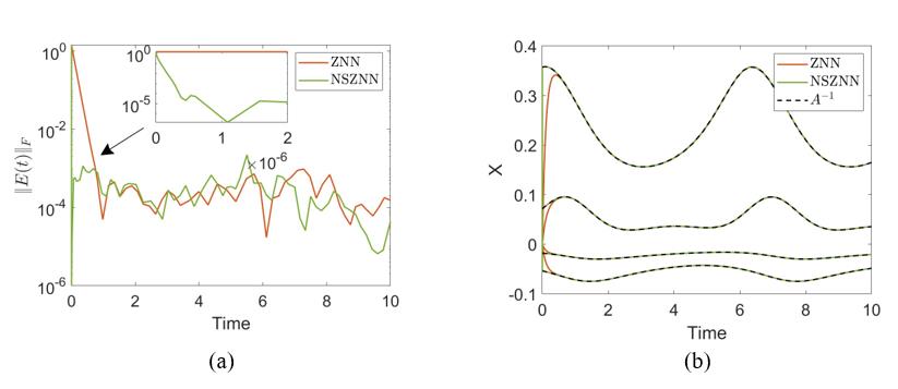
Experiment 1

The experiment deals with the next $\mathrm{2}\times \mathrm{2}$ input matrix:

$A\left(t\right)=\left[\begin{array}{ll}\mathrm{5}-\mathrm{2}\mathrm{c}\mathrm{o}\mathrm{s}\left(t\right)& -\mathrm{2}+\mathrm{c}\mathrm{o}\mathrm{s}\left(t\right)\\ \mathrm{4}+\mathrm{s}\mathrm{i}\mathrm{n}\left(\mathrm{2}t\right)& \mathrm{5}\mathrm{s}\mathrm{i}\mathrm{n}\left(t\right)-\mathrm{20}\end{array}\right].$

The outcomes of the ZNN and NSZNN dynamics for tackling the TV-MI problem are presented in Figure 1.

See Full Size >

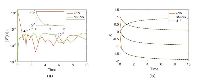
Experiment 2

This experiment deals with the following $\mathrm{5}\times \mathrm{5}$ input matrix:

$A\left(t\right)=\left[\begin{array}{lllll}t+\mathrm{1}& t& t& t& t\\ t& t-\mathrm{1}& t& t& t\\ t& t& t+\mathrm{1}& t& t\\ t& t& t& t-\mathrm{1}& t\\ t& t& t& t& t+\mathrm{1}\end{array}\right].$

The outcomes of the ZNN and NSZNN dynamical flows for tackling the TV-MI problem are presented in Figure 2.

See Full Size >

References

Cichocki, A., & Unbehauen, R. (1993). A Cochocki and Rolf Unbehauen. Neural networks for optimization and signal processing. John Wiley & Sons, Inc.
Dai, J., Chen, Y., Xiao, L., Jia, L., & He, Y. (2022). Design and Analysis of a Hybrid GNN-ZNN Model With a Fuzzy Adaptive Factor for Matrix Inversion. IEEE Transactions on Industrial Informatics, 18(4), 2434-2442. DOI:
Jin, L., Zhang, Y., Li, S., & Zhang, Y. (2017). Noise-Tolerant ZNN Models for Solving Time-Varying Zero-Finding Problems: A Control-Theoretic Approach. IEEE Transactions on Automatic Control, 62(2), 992-997. DOI:
Katsikis, V. N., Stanimirovic, P. S., Mourtas, S. D., Xiao, L., Karabasevic, D., & Stanujkic, D. (2022). Zeroing Neural Network With Fuzzy Parameter for Computing Pseudoinverse of Arbitrary Matrix. IEEE Transactions on Fuzzy Systems, 30(9), 3426-3435. DOI:
Smarandache, F. (2003). A unifying field in logics: Neutrosophic Logic. Neutrosophy, Neutrosophic Set, Neutrosophic Probability. American Research Press, Rehoboth.
Stanimirović, P. S., Mourtas, S. D., Katsikis, V. N., Kazakovtsev, L. A., & Krutikov, V. N. (2022). Recurrent Neural Network Models Based on Optimization Methods. Mathematics, 10(22), 4292. DOI:
Zadeh, L. A. (1965). Fuzzy sets. Information and Control, 8(3), 338-353. DOI:
Zhang, Y., & Ge, S. S. (2005). Design and Analysis of a General Recurrent Neural Network Model for Time-Varying Matrix Inversion. IEEE Transactions on Neural Networks, 16(6), 1477-1490. DOI:
Zhong, N., Huang, Q., Yang, S., Ouyang, F., & Zhang, Z. (2021). A Varying-Parameter Recurrent Neural Network Combined With Penalty Function for Solving Constrained Multi-Criteria Optimization Scheme for Redundant Robot Manipulators. IEEE Access, 9, 50810-50818. DOI: 10.1109/access.2021.3068731
Copyright information
This work is licensed under a Creative Commons Attribution-NonCommercial-NoDerivatives 4.0 International License
About this article
Publication Date
27 February 2023
Article Doi
eBook ISBN
978-1-80296-960-3
Publisher
European Publisher
Volume
1
Print ISBN (optional)
-
Edition Number
1st Edition
Pages
1-403
Subjects
Hybrid methods, modeling and optimization, complex systems, mathematical models, data mining, computational intelligence
Cite this article as:
Mourtas, S. D., Stanimirović, P. S., & Katsikis, V. N. (2023). A Neutrosophic Adaptive Recurrent Neural Network for Time-Varying Matrix Inversion. In P. Stanimorovic, A. A. Stupina, E. Semenkin, & I. V. Kovalev (Eds.), Hybrid Methods of Modeling and Optimization in Complex Systems, vol 1. European Proceedings of Computers and Technology (pp. 249-255). European Publisher. https://doi.org/10.15405/epct.23021.30