Application of Convolutional Neural Networks to Determine Induction Soldering Process Technological Stages

Abstract

Presented study focuses on solving the problem of controlling the technological process of induction soldering of spacecraft waveguide paths in terms of determining the stages of such a technological process based on the analysis of the video image from the soldering zone. The need to solve this problem lies in the features of the used sensors for optical control of the heating temperature of products. The accuracy of the pyrometer readings significantly affects both the quality of preparation of the surfaces of waveguide elements and the features of the soldering process itself. When the appearance of evaporation during the melting of the flux can significantly distort the temperature readings in soldering zone. In this situation, the precisely-set value of the heating process stabilization temperature, at which the solder melts and the joint is formed, may not correspond to the real temperature and cause the appearance of defects in the finished product, associated with insufficient flow of the solder or the appearance of burns. As a means to implement the technology of machine vision, the use of convolutional neural networks is proposed. This study considers the use of one of the popular architectures of such networks - DenseNet. To select the effective values of hyperparameters, a grid search with cross-validation was used. As a result, the model was obtained that allows to determine the stage of solder melting with an accuracy of over 0.99 on test and verification samples.

Keywords: Convolutional neural networks, automation, control, image recognition, DenseNet, induction soldering, waveguide path

Introduction

When fixed, the soldering process produces high-quality sealing seams that allow this technology to be applied in the space industry, in particular for the creation of waveguide tracts of spacecraft. Pyrometric sensors are widely used in the construction of systems for the automated control of induction soldering. However, the quality of their measurements is significantly affected by the quality of the waveguide elements’ surfaces preparation, and the features of the soldering process itself. For example, the appearance of evaporation during the melting of the flux can significantly distort the temperature readings in soldering zone.

In this situation, it is appropriate to determine the melting point of the solder not by the temperature of the pyrometers, but by analysing the video image from the soldering zone. Artificial intelligence techniques, namely artificial neural networks, have proven to be effective in solving these problems.

Thus, the aim of the work is to automate and improve the quality of the technological process of induction soldering through the introduction of a method for recognizing its technological stages using artificial neural networks.

Research Object

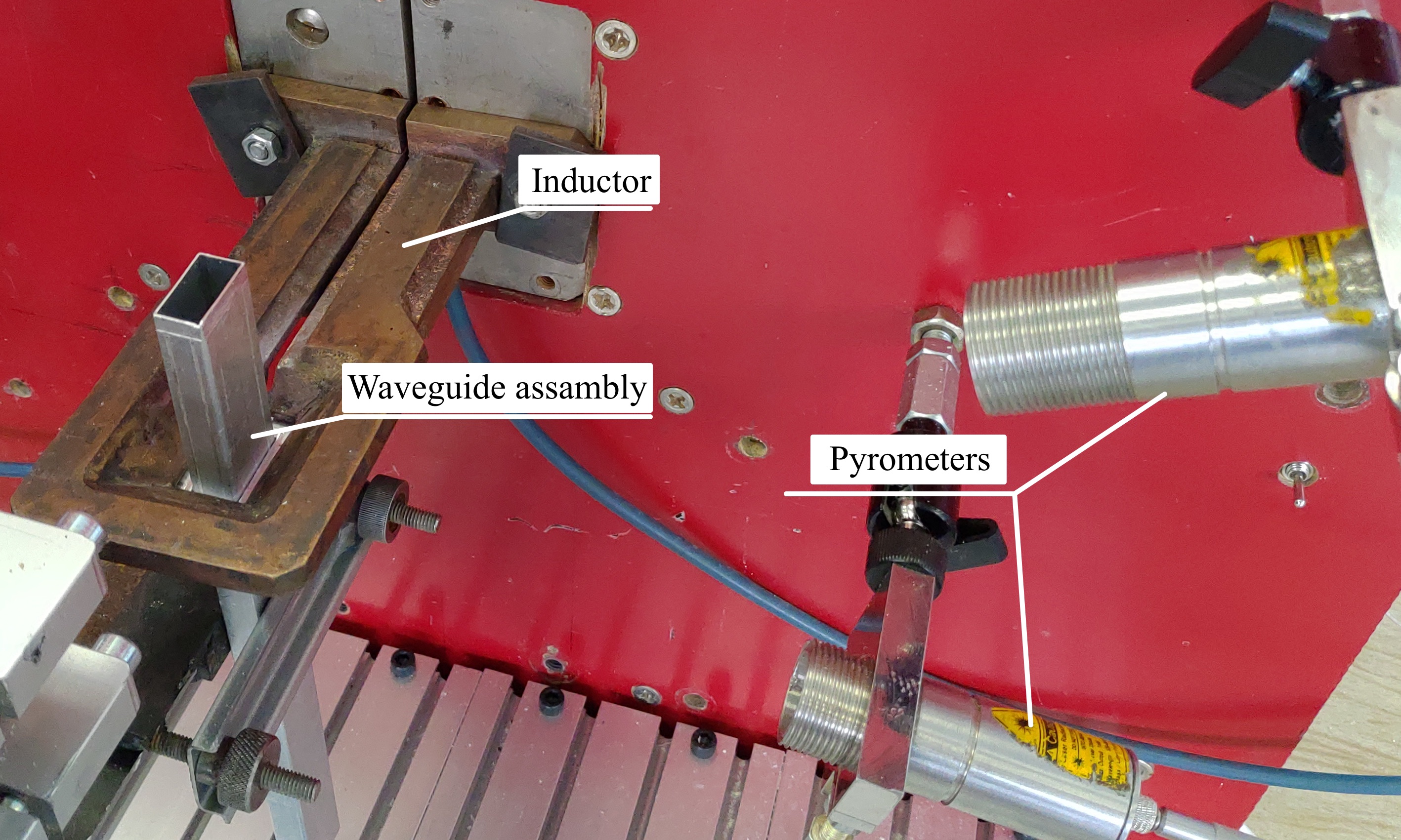
Induction soldering is the process of joining metals or non-metallic materials by melting the solder by induction heating produced by eddy currents inducted in parts. Inductors for installations are made of copper tubes, their shape depends on the configuration of the parts to be soldered (Figure 1).

See Full Size >

The use of induction soldering method is conditioned by the presence of unique advantages of this method of joining elements. Among them there are (Emilova & Tynchenko, 2016):

• Selective heating. Induction brazing is capable of heating a small area, corresponding to production tolerances. In this case, only those parts of the workpiece that are in the immediate vicinity of the connecting elements are heated.
• Quality of joints. The joints obtained by this method are pure hermetic seams.
• Reduction of oxidation. Induction heating does not cause such strong oxidation and scale on parts as classical soldering methods. This avoids costly cleaning procedures.
• Fast heating cycles. Using high concentration energy, it is possible to quickly heat parts to the soldering temperature.

However, in the majority of cases, in enterprises using induction brazing technology, the process is carried out manually by the operator, who monitors the heating process, visually determining the melting point of the solder and seam filling, At the same time being in the zone of vapours of fluxes and solids. The manual management of the soldering process does not ensure accurate compliance with the required heating modes and their repeatability, so the quality of the soldering depends largely on the skill of the contractor, i.e., underheating and overheating are possible and as a consequence of failure, deformation, warping and burning parts. All this leads to the formation of defects of brazed seams. Therefore, automation of the soldering process (Selevtsov, 2019) is necessary to ensure accurate performance of the soldering process, to eliminate the human factor and to ensure high quality of the soldering joints.

The works (Tynchenko et al., 2016; Tynchenko et al., 2019) offer systems for the automation of induction braking, based on the heating process control by changing the power supplied to the inductor, using the temperature information in the soldering zone.

The system is not without shortcomings. The automated induction soldering process described in this work uses many parameters that are filled automatically from the database, but the system is not ready to adapt to changes not related to temperature changes, which creates the possibility of distortion of information about the process. It is assumed that the result of the previously considered stages, for example, the flux dried or solder began to melt, is automatically considered to be achieved when the set temperature for these stages.

The main task is to determine the stage of soldering on the input image obtained by recording or processing the streaming video of the technological process, due to its characteristic features, this step can be classified as a separate part of the process. This solution would remove the operator’s subjectivity, the end result of which would be an improvement in the quality of the process.

It can be determined that the input data of the intelligent system to be developed will be an image (an array of pixels), obtained in the form of both a separate frame and a streaming video from the camera attached for monitoring the installation of induction soldering. As the output you need to get: the name/unique stage number, which corresponds to the input image.

Thus, the problem is reduced to processing the input image with computer vision. Feature descriptors are used to extract useful information and discard unnecessary information. The feature descriptor converts the original image from the format “Width×Height×Number of Channels” into an array of features “Width×Height×Number of Features” (Simonyan & Zisserman, 2014).

Research Methods

Image recognition methods

This section discusses the existing image recognition methods, as well as the advantages of methods based on deep learning, including artificial neural networks (Gulina & Kolyushkin, 2012).

The traditional image classifier, i.e., a non-deep learning classifier, contains the following steps:

• Image Input.
• Pre-processing of the input image.
• Feature extraction: Haar traits, histogram of directional gradients. Scaled invariant feature transformation and reliable element acceleration.
• Learning/classification algorithm
• Tagging.

The input image may contain a large amount of redundant information that will not be required in the classification and will ultimately affect the algorithm’s performance. At the feature extraction stage, the amount of unnecessary information contained in the image is reduced by discarding irrelevant features.

Learning algorithms consider feature vectors as points in higher dimension space, and attempt to find planes/surfaces that separate higher dimension space in such a way that all examples belonging to the same class, are on the same side of the plane/surface. The trained algorithm will be able to match the input image to a certain class.

Based on the results of the classification, a label is assigned to the image reflecting its class.

Viola-Jones method

This method is based on the integral representation of the image, the method of constructing the classifier based on the adaptive boosting algorithm (AdaBoost) and the method of combining the classifiers into a cascade structure.

The simplified design of the algorithm is as follows: before recognition, the test image learning algorithm learns a classifier consisting of the values of certain features. The algorithm then searches for objects on different scales of the image, based on a trained classifier. The output of the algorithm gives many found objects on different scales.

The fundamental idea of the Viola-Jones algorithm for object recognition is to isolate local features (features) of the image and then train the algorithm on them. The search on the image is done according to the principle of the scanning window - the image is scanned by the search window, and the classifier is applied at each position of the window (Tymchuk, 2017).

Histogram of oriented gradients (HOG)

The histogram descriptor of directed gradients is computed by filtering the original image using kernels [ $-$1, 0, 1] and ${[-1,0,1]}^T$. The size and direction of gradients are determined by Equations (1) and (2):

$g=\sqrt{g_x^{\mathrm{2}}+g_y^{\mathrm{2}}}$ (1)

$\theta =arctan\frac{g_x}{g_y}$(2)

where - gradient, - abcisse axis gradient, - ordinate axis gradient, - direction of gradients.

Gradient with index “x” appears on vertical lines, with index “y” on horizontal lines.

In each pixel, the gradient has a magnitude and a direction. For color images, the gradients of the three channels are estimated. The magnitude of a gradient in a pixel is the maximum value of the gradients of the three channels, and the angle is the angle corresponding to the maximum gradient.

The next step is to compute the histogram of the gradients in cells. The selected image fragment is divided into blocks of size n×n pixels. For example, in the work of Dalal and Triggs (2005), optimal block sizes have been determined as 16×16 and 8×8, as well as 9 histogram channels, taking into account the fact that these block sizes are considered optimal for the initial problem of pedestrian detection.

Methods based on deep learning

In-depth learning is a set of machine learning methods based on the learning of representations, rather than specialized algorithms for solving narrowly oriented problems. As for artificial neural networks (ANN) are computational systems based on the principles of biological neural networks that make up the brain of animals. Such systems are able to gradually improve their ability to perform tasks, usually without programming for specific tasks. For example, by recognizing images of cats, they can learn to recognize images that contain cats by analyzing examples of images that have been manually labeled as “cat” or “no cat”, and using the analysis results to identify cats in other images.

Sometime after HOG, a new, much more efficient and powerful image recognition method was introduced, using deep learning.

Figure 2 presents the algorithm results (as a percentage of the top 5 error) at the ImageNet Large Scale Visual Recognition Challenge (ILSVRC) from 2010 to 2015. In this case, the top 5 error rate is the proportion of test images for which the correct label is not among the five labels that the algorithm considers most likely. This feature is due to the fact that the databases used for training may be present at once several objects, while only one of them is annotated.

See Full Size >

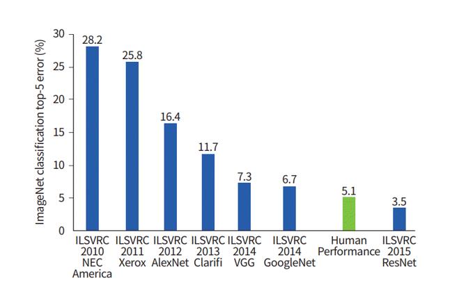
Since 2012, models other than artificial neural networks have not won the competition. There are a large number of architectures that are faster and at the same time deeper than AlexNet, improving the accuracy of image classification: GoogleNet, Inception, ResNet, as well as the networks originating from and that are their combinations. At the moment, INS is not only the most effective, but also the most flexible tool for image recognition.

Artificial neural networks

In artificial neural networks (ANN) a neuron is a basic unit of information processing. The model of a neuron is shown in Figure 3.

See Full Size >

This model includes synaptic connections, input adder, activation function, and threshold element.

Synaptic connections connect neurons. Each connection is characterized by a weight (), which is also referred to in some sources as the force of communication. The signal at the synapse input associated with the neuron is multiplied by the weight. The weights are indexed as follows: the first index corresponds to the neuron in question, the second input to the end of the synapse associated with the weight. Synaptic weight of ANN can take both positive and negative values.

The adder completes (a linear combination) of all signals weighted relative to existing neuron synapses. The activation function then brings the output signal amplitude to some normalized range. This range is usually in the range [0, 1] or [-1, 1].

The model of this neuron is described by the following pair of equations:

$u_j=\mathrm{}\underset{i=\mathrm{1}}{\overset{n}{\sum }}{w}_{ij}{x}_i$(3)

$o_j=\phi (u_j+{\theta }_j)$(4)

where – input signals; – synaptic weight neuron; – linear combination of inputs; – threshold; $\phi$ – activation function; – neuron output signal. Postsynaptic potential is obtained by the equation:

${net}_j=\mathrm{}{u}_j+{\theta }_j$(5)

Convolutional neural network

The Convoluted Neural Network (CNN) is an artificial neural network architecture aimed at effective pattern recognition and part of deep learning technologies. The main difference between CNN and conventional approaches to image recognition is the ability to independently extract features from input data. That is, there is no need to create attributes for each individual task.

The operation of these neural networks is based on the principle of the visual zone of the brain, whereby individual neurons respond to stimuli only in a limited area of the visual field called the receptive field. Such fields overlap each other, covering the entire field of view (Liu et al., 2017).

CNN provides advanced ways of solving computer vision problems using a universal, scalable, self-contained approach that can be applied to different subject areas without having to know anything about them. You don’t need to create the traits yourself anymore, because the neural network itself learns to extract useful traits with enough training and data (Ding & Tao, 2017; Ordóñez & Roggen, 2016).

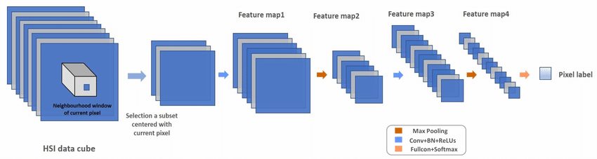
Convolution neural networks are characterized by the presence of convolution layers (i.e., convolution) and sub-samples (pooling). The combination of these layers is a feature extractor. Extractors extract first low-level features (e.g., contours and lines), then medium-level (shapes and combinations of several low-level features) and finally high-level features. The typical architecture of the convolution network feature extractor is shown in Figure 4. The layers of the convolution and sub-sample are usually followed by a fully connected layer, acting as a classifier.

See Full Size >

CNN DenseNet

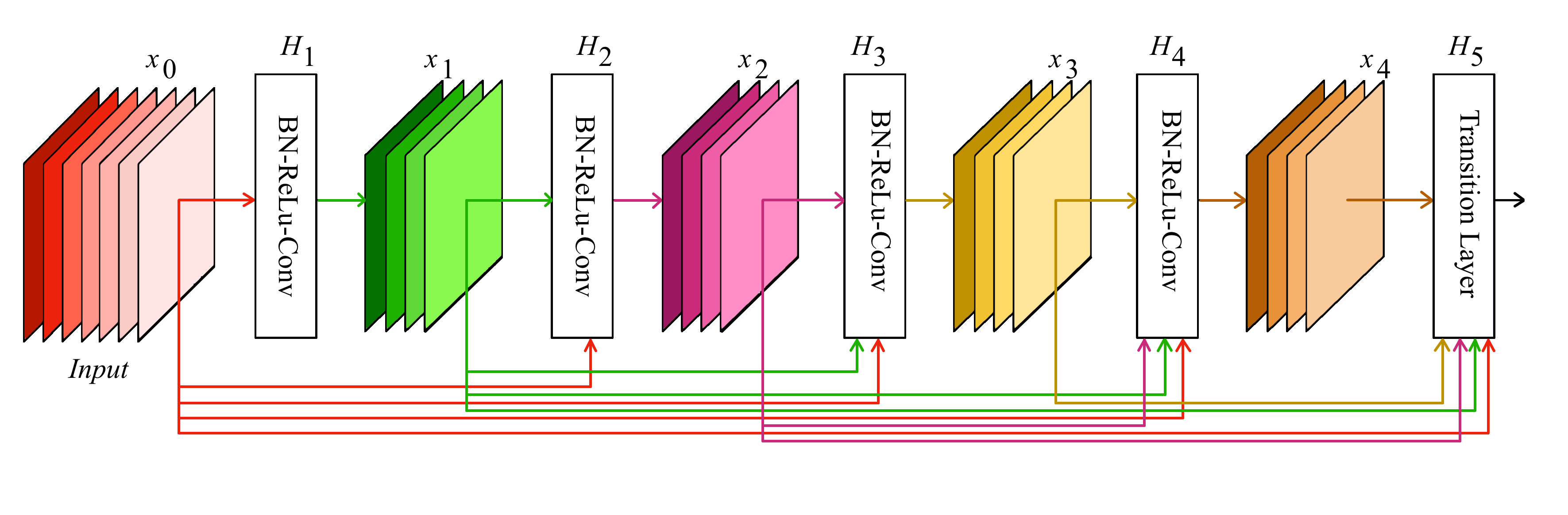
Densely Connected Convolutional Network, abbreviated DenseNet, was proposed in 2017. As seen from the example of the networks considered earlier, the success of ResNet has prompted the introduction of identity bypass connections to create deeper neural networks (Khan et al., 2020; Liu et al., 2017). DenseNet is based on a fully connected (Dense) block in which the output of each layer is transferred to each of the subsequent layers. In this case, the transfer of information occurs at the expense of concatenation, not summation, as in ResNet. The fully connected block can be seen in the Figure 5.

See Full Size >

DenseNet performs well on small datasets, so will be tested as part of this work.

Findings

For the operation was used a computer running Windows OS with the Intel Core i5-9400 processor, as well as a graphics card Nvidia GeForce 1060 with 6 GB of memory of the graphic critic.

Software used in the implementation:

• Visual Studio Code with Jupyter Notebook extension.
• Python programming language (version 3.9) as part of Anaconda (Conda core) (Raska, 2022; Sharden et al., 2022).
• Image library of OpenCV.
• Library ScikitLearn.
• Library for machine learning and working with TensorFlow tensors.
• Keras API is a TensorFlow package for creating neural network models.
• In addition, the Nvidia CUDA and cuDNN software was used to use the graphical accelerator in training.

TensorFlow and its Keras APIs are the most popular tools for creating neural networks at the moment.

Experimental studies

During the review of the architectures of convoluted neural networks, various variants studied in the previous sections were considered, such as VGGnet, Xception, ResNet, MobileNet, etc. The available data set was tested to determine the most appropriate models. When selecting for the pool of testing preference was given to the following criteria (Golubinsky & Tolstoy, 2018):

• Number of parameters – increasing the number of parameters increases the computational cost and the required amount of memory of the graphical accelerator.
• Its is possible to work with small amounts of data because there are no ready datasets for this task, and creating your own sample does not achieve the desired number of images for each class.
• The relative novelty of the model – its makes no sense to use the old models when they have their newer counterparts, surpassing them in computational efficiency and classification accuracy.
• Popularity – The more popular the architecture, the easier its is to find related documentation and implementation examples.

Within the framework of research, various parameters of learning and images have changed:

• Number of epochs (10, 15, 20, 25).
• Image size. Smaller image size helps speed up network learning, but makes its harder to extract features. Networks such as VGG or DenseNet by default accept 224224 resolution images, EfficientNetB2 accepts 260260 size images, xResNet receives 254254 size images, Xception – 299299 size images.
• Optimizers Adam (adaptive moment estimation), SGD (stochastic gradient descent), and some RMSProp networks have been tested.
• Learning speed (10-3, 10-4, 10-5).
• The package size is 16.

The results of the study are collected in Table 1.

Effective hyperparameter values were selected using the GridSearchCV utility based on the probability of correct stage classification (accuracy) and stability of convergence.

See Full Size >

DenseNet has a tendency to achieve very high accuracy very quickly, and after ten eras of training its accuracy exceeded 90 percent in most cases. This high accuracy of the classification is due to the large number of similarities in the images, which, despite the data augmentation, affects its retraining. In order to address this problem, it is proposed to further increase the data set with different angles and types of blanks.

The learning process is depicted in Figure 6. The training of the model took place over 15 epochs of 156 packages, 16 images each.

See Full Size >

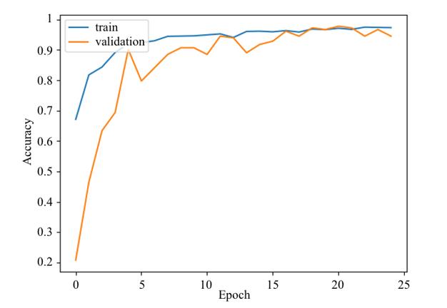
Adam was selected as the optimizer with a learning rate = 0.0001. Categorical cross-entropy was used as the loss function. The maximum accuracy was 0.9952, on the test sample - 0.9945.

An average of 56-57 seconds was required for one training era.

Conclusion

In the course of the study, an analysis of the subject area was performed, in the course of which the need for automation of visual observation of the induction soldering process was identified.

An analytical review of the methods of classifying images, including the Viola-Jones method, the histograms of directional gradients, artificial neural networks, revealed such advantages of neural networks, as high accuracy and versatility due to the ability to independently extract signs.

In the preparation of the training sample from the different video of induction the frames were extracted, which were assigned markered classes corresponding to the stages of the technological process. The images were divided into training and validation samples with a ratio of 93/7. Then the images from the training sample were augmented. For each second image of the sample one of the following transformations was applied: 15% scaling of the random area, rotating the image to a corner, multiples 90 degrees, image shift by 20%.

As a result of the experimental analysis of the application of architecture of convoluted neural networks DenseNet169 was shown its effectiveness for the solution of the task - accuracy was more than 99%.

The further direction of research is the study of the application of other popular architectures of convoluted neural networks, as well as the integration of a module for determining the stages of the technological process of induction braking into an automated control system.

Acknowledgments

This work was supported by the Ministry of Science and Higher Education of the Russian Federation (Grant No.075-15-2022-1121).

References

• Dalal, N., & Triggs, B. (2005). Histograms of oriented gradients for human detection. In 2005 IEEE computer society conference on computer vision and pattern recognition (CVPR'05) (Vol. 1, pp. 886-893). IEEE. DOI:

  Google Scholar

  Crossref

• Dao, T., Gu, A., Ratner, A., Smith, V., De Sa, C., & Ré, C. (2019). A kernel theory of modern data augmentation. In International Conference on Machine Learning (pp. 1528-1537). PMLR.

• Ding, C., & Tao, D. (2017). Trunk-branch ensemble convolutional neural networks for video-based face recognition. IEEE transactions on pattern analysis and machine intelligence, 40(4), 1002-1014. DOI:

  Google Scholar

  Crossref

• Emilova, O. A., & Tynchenko, V. S. (2016). Induction braking: process and its features. Reshetnevsky readings, 2(20), 173-174.

• Golubinsky, A. N., & Tolstoy, A. A. (2018). Choice of architecture of artificial neural network based on comparison of efficiency of image recognition methods. Herald of the Voronezh Institute of the Russian Ministry of Internal Affairs, 1(1), 27-37.

• Gulina, Y. S., & Kolyushkin, V. Y. (2012). Method of calculation of probability of image recognition by the human operator. Messenger of the Moscow State Technical University. NE Bauman. Series «Instrument Making», 1(1), 100-107.

• Khan, A., Sohail, A., Zahoora, U., & Qureshi, A. S. (2020). A survey of the recent architectures of deep convolutional neural networks. Artificial intelligence review, 53(8), 5455-5516. DOI:

  Google Scholar

  Crossref

• Liu, W., Wang, Z., Liu, X., Zeng, N., Liu, Y., & Alsaadi, F. E. (2017). A survey of deep neural network architectures and their applications. Neurocomputing, 234, 11-26. DOI:

  Google Scholar

  Crossref

• Ordóñez, F. J., & Roggen, D. (2016). Deep convolutional and lstm recurrent neural networks for multimodal wearable activity recognition. Sensorsi, 16(1), 115. DOI:

  Google Scholar

  Crossref

• Raska, C. (2022). Python and machine learning. Litres.

• Selevtsov, L. I. (2019). Automation of technological processes. Moscow Academia.

• Sharden, B., Massaron, L., & Boscetti, A. (2022). Large-scale machine learning together with Python. Litres.

• Simonyan, K., & Zisserman, A. (2014). Very deep convolutional networks for large-scale image recognition. arXiv preprint arXiv:1409.1556, 1, 1-14.

• Tymchuk, A. (2017). Viola-Jones method for recognition of objects in the image. Modern science: actual problems of theory and practice. Series: Natural and Technical Sciences, 1(6), 63-68.

• Tynchenko, V. S., Bocharov, A. N., Laptenok, V. D., Seryogin, Y. N., & Zlobin, S. K. (2016). Software of technological process of soldering waveguide paths of spacecraft. Software products and systems, 2(114), 128-134. DOI:

  Google Scholar

  Crossref

• Tynchenko, V. S., Laptenok, V. D., Petrenko, V. E., Murygin, A. V., & Milov, A. V. (2019). Induction soldering automation system based on two control circuits with workpiece positioning. Software and systems, 32(1), 167-173. DOI:

  Google Scholar

  Crossref